A guest article by Nicholas Lewis
Note: This is a long article: a summary is available here.
Introduction
In a recent paper[1], NASA scientists led by Kate Marvel and Gavin Schmidt derive the global mean surface temperature (GMST) response of the GISS-E2-R climate model to different types of forcing. They do this by simulations over the historical period (1850–2005) driven by individual forcings, and by all forcings together, the latter referred to as the ‘Historical’ simulation.
They assert that their results imply that estimates of the transient climate response (TCR) and equilibrium climate sensitivity (ECS) derived from recent observations are biased low.
Marvel et al. use the GISS-E2-R historical period simulation responses to revise estimates of the transient climate response (TCR) and equilibrium climate sensitivity (ECS) from three observationally-based studies: Otto et al. 2013, Lewis and Curry 2014 and Shindell 2014. Their revisions give figures that are substantially higher than in the original studies. Remarkably, the Marvel et al. reworked observational estimates for TCR and ECS are, taking the averages for the three studies, substantially higher than the equivalent figures for the GISS-E2-R model itself, despite the model exhibiting faster warming than the real climate system. Not only is the GMST increase simulated by GISS-E2-R is higher than that observed, but the ocean heat uptake rate is well above the observed level.[2] No explanation is given for this surprising result.
The press release for the paper quotes Kate Marvel as follows:
‘Take sulfate aerosols, which are created from burning fossil fuels and contribute to atmospheric cooling,’ she said. ‘They are more or less confined to the northern hemisphere, where most of us live and emit pollution. There’s more land in the northern hemisphere, and land reacts quicker than the ocean does to these atmospheric changes.’
and continues by saying:
‘Because earlier studies do not account for what amounts to a net cooling effect for parts of the northern hemisphere, predictions for TCR and ECS have been lower than they should be.’
However, this is not true when the effective radiative forcing (ERF) measure of aerosol forcing – preferred by IPCC AR5 and used in the observational studies Marvel et al. criticises – is employed. When calculated correctly using Marvel et al.’s data, bases and assumptions, aerosol ERF had a transient efficacy of 0.97 – almost the same as the 0.95 for GHG forcing and 1.00 for CO2 forcing. This result is in line with the findings in Hansen 2005.This implies that aerosol forcing has had almost the same effect on GMST since 1850, relative to its ERF, as did CO2 and GHG forcing. Its concentration in the northern hemisphere did not lead to a greater cooling effect globally since 1850.
Studies like Marvel et al. can be valuable in showing the effects of differing forcing agents in climate models, which – if similar across climate models – may provide a guide to their effects in the real climate system. Unfortunately, I believe that the Marvel et al. results are substantially inaccurate and misleading. Its conclusions are therefore unfounded. But, as with any single-model study, even were its results unimpeachable they would reflect the behaviour of the particular model involved, which may be very different from that of other models and, more importantly, from that of the real climate system.
Background
It is known that an equal radiative forcing caused by different agents may have a greater or lesser effect on GMST. That is to say, different types of forcing may have different ‘efficacies’. The efficacy of a forcing is defined as its effect on GMST relative to that of the same amount of forcing by CO2. The efficacy of CO2 forcing is therefore one. This definition is reasonable: CO2 is the dominant greenhouse gas and TCR and ECS are measures of the GMST response – respectively after 70 years of linearly increasing forcing, and after the ocean reaches equilibrium – to a doubling of CO2 concentration. The forcing–efficacy framework, to be useful, requires that GMST response scales linearly with forcing and that the GMST response to a mixture of different forcings equals the sum of the responses to the constituent individual forcings. Both these assumptions typically hold quite well in general circulation models (GCMs).
A seminal paper[3] lead authored by James Hansen of GISS (henceforth Hansen 2005), based on simulations by a previous version of the GISS GCM, Model E, estimated efficacies for different forcing agents. Hansen 2005, a commendably thorough paper, advanced climate science and helped pave the way for the use of effective radiative forcing (ERF) in IPCC AR5. Hansen 2005 derived efficacies in terms of both the instantaneous radiative flux change at the tropopause (iRF or Fi) and the flux change after the stratosphere has adjusted to the forcing (RF or Fa). RF is the same whether measured at the tropopause or the top-of-atmosphere (TOA). Hansen also derived efficacies relative to Fs, the TOA flux change with sea surface temperature (SST) held fixed, and Fs*, an approximation to Fs derived by regressing TOA flux on GMST following a step change in forcing, in a so-called Gregory plot, in this case for 10–30 years. Hansen’s Fs was adjusted for the change in land surface temperatures that occurs when forcing is changed but SST is held fixed.
Section 8.1 of AR5[4] gives a useful introduction to radiative forcing in its different variants. It defines ERF similarly to Hansen’s Fs, but with no adjustment made for the change in land temperature (which is modest when SST is fixed), and notes that ERF can also be estimated by regression, as for Fs*. The ERF, Fs and Fs* measures allow for the troposphere to adjust to the imposed forcing, as well as the stratosphere.
Hansen 2005 found that although when iRF was used to measure forcing, the efficacy of some forcing agents differed substantially from one, when either Fs and Fs* were used efficacies were close to one for almost all types of forcing investigated.
Further details of Hansen 2005’s findings, and information on relevant other studies are given in Appendix A.
Marvel et al.’s investigation of forcing efficacies
Marvel et al. used the newer E2-R version of the GISS model to carry out single-forcing simulations similar to those in Hansen 2005. However the set of simulations was more limited in scope and forcings were made to follow their estimated historical evolution from 1850 to 2005 rather than being imposed in full at the start of the simulation.
Forcings, in iRF terms, were derived each year by radiation-only calculations, with the forcing agent evolving but all other variables held at preindustrial (1850) values. ERFs were estimated only for the year 2000, from simulations with the then level of the forcing agent concerned and only SSTs fixed at 1850 values. Equilibrium and transient efficacies, and TCR and ECS estimates, were derived by comparing the historical GMST response (ΔT) with the causative forcing change (ΔF) respectively with and without the associated change in ocean heat uptake rate (ΔQ) deducted. The decadal mean ΔT, ΔF and ΔF−ΔQ values used are all anomalies relative to drift-adjusted quasi-equilibrium preindustrial control runs, from which these simulations were spawned in 1850. The mean ΔT and ΔQ values from an ensemble of five runs were used.
Specifically, the relationships between decadal means of ΔT and ΔF (for TCR) or ΔF − ΔQ (for ECS) in each forced simulation are used to produce separate estimates of GISS-E2-R’s TCR and ECS for each forcing agent, according to the energy budget equations:[5]
![]() where F2xCO2 is the forcing from a doubling of CO2 concentration. For ERF the ratios are simply quotients based on 1996–2005 values. For iRF, where values for all decades are available, the quotients that Marvel et al. use are the slopes of the best-fit lines when regressing ΔT using 1906–15 to 1996–2005 values. Marvel et al. calculate the transient (equilibrium) efficacy for each forcing as the ratio of the TCR (ECS) estimate it gives rise to divided by the actual, CO2 forced, values for GISS-E2-R, being 1.4°C for TCR and 2.3°C for ECS. Hansen 2005 instead derived transient efficacies (not equilibrium efficacies as stated by Marvel et al.) by directly comparing the ΔT/ΔF ratio for each forcing agent with that for CO2, in simulations with identical forcing time-profiles.
where F2xCO2 is the forcing from a doubling of CO2 concentration. For ERF the ratios are simply quotients based on 1996–2005 values. For iRF, where values for all decades are available, the quotients that Marvel et al. use are the slopes of the best-fit lines when regressing ΔT using 1906–15 to 1996–2005 values. Marvel et al. calculate the transient (equilibrium) efficacy for each forcing as the ratio of the TCR (ECS) estimate it gives rise to divided by the actual, CO2 forced, values for GISS-E2-R, being 1.4°C for TCR and 2.3°C for ECS. Hansen 2005 instead derived transient efficacies (not equilibrium efficacies as stated by Marvel et al.) by directly comparing the ΔT/ΔF ratio for each forcing agent with that for CO2, in simulations with identical forcing time-profiles.
In the ECS energy budget equation, ΔQ should be the TOA radiative imbalance (ΔN); Marvel et al. use the rate of ocean heat uptake (OHU) as an approximation to ΔN.
Marvel et al. state that in these equations F2xCO2 is taken as having an iRF of 4.1 W/m2; the ERF value used is not stated. Having derived efficacies for individual forcing agents, they then use them to re-estimate climate sensitivity from observed historical warming, using data for three previous studies and arriving at higher estimates than in those studies.
Figure 1 reproduces Figure 1a of Marvel et al., which shows the relationship in GISS-E2-R between changes ΔT in simulated GMST and ΔF in forcing, for six individual forcing agents as they are estimated to have evolved since 1850 and for the Historical simulations (all-forcings together, 6 runs). The forcing agents are long-lived greenhouse gases (GHG), anthropogenic aerosols (AA), land-use changes (LU), ozone (Oz), solar (SI) and volcanoes (VI). The filled circles are with forcing measured by iRF, and show means for decades ending from 1906–15 to 1996–2005. The open circles are for 1996–2005 mean GMST changes with forcing measured by ERF in 2000; the ΔT values are the same as for iRF.
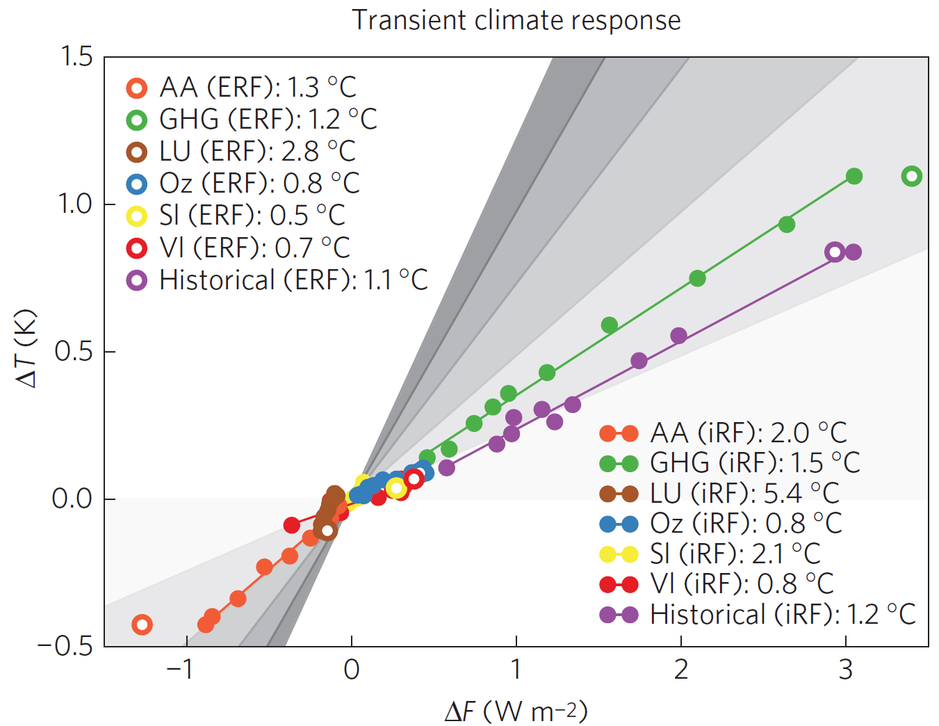 Figure 1: Reproduction of Figure 1a of Marvel et al.
Figure 2 reproduces Figure 1b of Marvel et al. It differs from Figure 1 only in that the x-axis shows ΔF−ΔQ rather than ΔF, as here equilibrium rather than transient sensitivity (and hence efficacy) is being estimated.
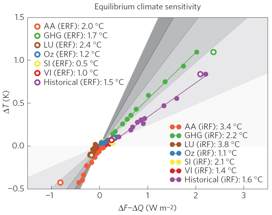 Figure 2: Reproduction of Figure 1b of Marvel et al.
Fundamental problems with Marvel et al.’s estimation of forcing efficacies, TCR and ECS
There are at least six fundamental problems with Marvel et al. estimation methodology and its implementation, apart from the fact that the estimates relate to the behaviour of GISS-E2-R model, not the real world.
- What is primarily relevant for observational estimates of climate sensitivity based on changes over the historical period is how much forcing and warming recent levels of different forcing agents generate in today’s climate state, relative to the preindustrial (1850) state of affairs. By contrast, Marvel et al. estimate the forcing and resulting warming produced in the preindustrial climate system when it is altered in one respect only: the concentration of a single forcing agent. For non-GHG forcing agents, this leaves the climate in a near preindustrial, or colder climate state, not close to today’s climate state. In GISS-E2-R these two situations can, at least for certain agents, give rise to very different levels of forcing, whether or not they do so in reality; it is unclear to what extent the GMST responses in the two cases will reflect their different measured forcings.For example, in GISS-E2-R the 2000 level of anthropogenic aerosol loading produces direct aerosol TOA radiative forcing of –0.40 W/m2 in the 2000 climate, but zero forcing in the 1850 climate.[6] Also, ozone iRF forcing in GISS-E2-R differs when the climate state is allowed to evolve as in the all-forcings simulation: 0.28 W/m2 in 2000 versus 0.45 W/m2 per Marvel et al.’s value based on an approximately preindustrial climate state.21 This shows that for some forcing agents Marvel et al.’s methodology does not correctly quantify forcing in GISS-E2-R for recent decades of the Historical simulation, making its related efficacy and sensitivity estimates very doubtful.
- The energy budget equation for ECS actually estimates effective climate sensitivity for the timescale over which changes are measured, which only equals equilibrium climate sensitivity if feedbacks do not vary with time.[7] However, effective climate sensitivity in GISS-E2-R increases with time since the forcing was applied, as in many GCMs. Efficacy is defined as a forcing agent’s effect on GMST relative to that of the same forcing from CO2. That implies GISS-E2-R’s effective climate sensitivity to CO2 forcing over a timescale equivalent to the historical evolution of the forcing concerned, not its equilibrium climate sensitivity, must be used when estimating equilibrium efficacy for a forcing agent, and as a comparator for the ECS estimate it generates.The effective climate sensitivity of GISS-E2-R over such an equivalent timescale is only 1.9–2.0°C, well below its ECS of 2.3°C.[8] By using the model ECS value of 2.3°C rather than its effective sensitivity, the Marvel et al. method substantially underestimates equilibrium efficacies for all types of forcings considered. Applying the same methodology to CO2 yields the absurd result that CO2 has an efficacy of less than one when compared to its own performance.
- It is doubtful whether Marvel et al. have used the correct GISS-E2-R F2xCO2 value for iRF and/or ERF calculations. Any error in the F2xCO2 value affects all estimated efficacies and sensitivities. See under the separate iRF and ERF estimates sections. Moreover, radiative transfer computation in GISS-E2 may be inaccurate; there is an unexplained discrepancy between its GHG forcing and that in ModelE, resulting in a GHG forcing level that is way out of line with IPCC estimates.[9]
- Marvel et al.’s use of ocean heat rather than TOA radiative imbalance data, which it is difficult to see any valid reason for, biases down its estimates of equilibrium efficacies and of ECS for the various forcings. Non-ocean components of the TOA radiative imbalance, ignored in Marvel et al. but allowed for in the observational studies it criticises, appear to contribute ~14% of the total imbalance in GISS-E2-R, so the ΔQ values used should all be divided by ~0.86 to obtain ΔN. Doing so increases most of the equilibrium estimates, typically by 5–10%.[10]
- The regression-with-intercept estimation method Marvel et al. use for iRF efficacies and sensitivities is inappropriate; and most of their estimates using ERF do not agree with the underlying data.
- Although Marvel et al. states that forcings and temperatures from the single-forcing runs add linearly, and that their vector sum does not differ substantially from the historical values, this is only very approximately true, as shown by the gaps between the purple arrows and circles in Figure 3, a reproduction of Figure 1c of Marvel et al. The differences are ~10% for ΔT and iRF ΔF values per the data. For unknown reasons, both plotted iRF ΔF values are shifted by approaching 10% relative to the data.[11]

Figure 3: Reproduction of Figure 1c of Marvel et al.
As Figure 4 shows, the difference between Historical iRF and the sum of the six separate forcings closely matches, within 0.02 W/m2 in every year, SnowAlbedo_BC iRF (understood to be included in the Historical simulations) minus LU iRF. So, the difference might conceivably be due to LU iRF being missing from the Historical iRF values. If so, that would depress the efficacy estimates for Historical iRF.
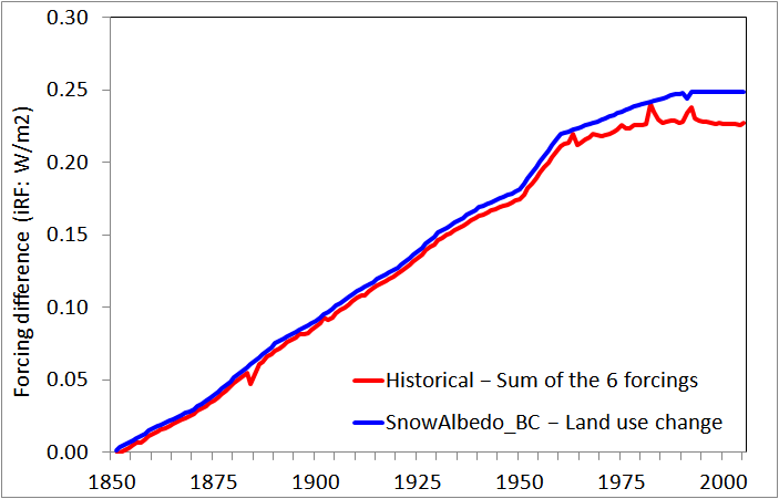
Figure 4: Differences hinting that LU iRF might be omitted from Historical forcing
Efficacy and sensitivity estimates based on iRF
Marvel et al.’s findings using iRF are a) largely irrelevant; and b) use an inappropriate estimation method. They may also use the wrong value for F2xCO2. The iRF data used is available here.
The findings using iRF are largely irrelevant because iRF is little used in observational studies, which generally use ERF and/or RF values.[12] It is therefore of little significance what efficacy, TCR and ECS estimates based on iRF values are. Marvel et al. seem to think that the IPCC AR5 RF values are iRFs, supporting their assertion that there is some ambiguity in the IPCC AR5 forcing definitions by writing: ‘For example, the best-estimate 1750–2011 iRF and ERF values given by the IPCC are identical, except for aerosols’. However, it is clear that the IPCC used RF, not iRF, values: there is no ambiguity on that point.[13] Hansen 2005 found that iRF was 56% higher than RF for ozone, 10% higher for CO2, and 5% higher for GHG and aerosols. Moreover, it is well known that, where they differ, ERF is a more appropriate measure than RF of the effect of forcings on GMST.[14] In particular, use of RF (or, a fortiori, iRF) for indirect aerosol forcing [giving RFaci] is inappropriate.[15] All three observational studies examined in Marvel et al. used ERF as a measure of aerosol forcing. Otto et al. and Lewis and Curry used ERF for non-aerosol forcings as well. None of the studies appear to have used iRF for any forcing.
The regression-with-intercept method used by Marvel et al. to estimate iRF efficacies and sensitivities is inappropriate since, although in all the simulations ΔT, ΔF and ΔQ each started at zero in 1850, in several cases the best-fit lines do not pass through or near the origin, implying that a zero forcing causes a material GMST change. That is unphysical. When either the ratio of changes since preindustrial in GMST and iRF are used instead of regression, as for ERF, or the regression best-fit lines are required to pass through the origin, substantially different iRF efficacy estimates are obtained for the forcings for land-use change, ozone, solar and volcanoes.[16]
The measure of F2xCO2 used by Marvel et al. for iRF, stated to be the model iRF value for CO2 doubling, appears instead to be the RF value in the GISS-E2-R model. Marvel et al. cites Hansen 2005 in support, but that gives values for the earlier GISS ModelE. Moreover, Hansen 2005 shows that in that model the iRF value was 10% higher, at 4.52 W/m2, than the RF value of 4.12 W/m2. The RF for doubled CO2 in the GISS E2 models is 4.1 W/m2;[17] I cannot find a published iRF value. If F2xCO2 is 10% higher in iRF than in RF terms in GISS ModelE2, as it was in GISS ModelE, then all Marvel et al.’s iRF efficacy, TCR and ECS estimates should be 10% higher.
In passing, I note that in Marvel et al.’s Figure 1 the iRF for volcanoes appears to have been shifted by +0.29 W/m2 relative to the data. No mention of this adjustment is made; the reason for it is unknown. It is unclear if it affects other results in Marvel et al.
Efficacy and sensitivity estimates based on ERF
All the ERF efficacy, TCR and ECS estimates depend on the ERF value for F2xCO2 in GISS-E2-R. Marvel et al. do not state this value and I cannot find a published value. However, giving a single set of TCR and ECS isolines for iRF and ERF in their Figure 1 implies that the same F2xCO2 value is used for both. I have therefore assumed that F2xCO2 for ERF in Marvel et al. is the same as it is for iRF, at 4.1 W/m2. However, it is arguable that the correct value is more probably ~4.5 W/m2.[18] If that is the case, all the ERF efficacy, TCR and ECS estimates should be 10% higher.
Tables 1 and 2 reproduce respectively the mean transient and equilibrium ERF efficacies stated in Table 1 of the Marvel et al. Supplementary Information (SI), along with the values I calculate from their 1996–2005 GMST data, averaged ERF data for 2000 and ocean heat uptake data (taking the trend over 1996–2005), and alternatively by accurately digitising ERF ΔF and ΔF−ΔQ values in Marvel et al. Figure 1.[19] I also show the effect of revising the ERF F2xCO2 value from 4.1 to 4.5 W/m2. For transient ERF efficacies, the relevant values from Hansen 2005 are shown for comparison. In the final row, iRF efficacies are shown to highlight where differences between ERF and iRF measures arise; a zero-intercept has been imposed when deriving the regression slopes, but no change made to Marvel et al.’s iRF F2xCO2 value.
Table 1 Transient efficacies per Marvel et al and other sources
| Forcing agent/ Source of efficacy estimates |
Aerosol AA |
Greenhouse gases GHG | Land-use change LU | Ozone Oz |
Solar SI |
Volcanoes VI |
Historical |
| Fig.1a ΔF | 0.97 | 0.95 | 2.23 | 0.62 | 0.42 | 0.53 | 0.84 |
| SI Table 1 | 0.83 | Not given | 1.81 | 0.53 | 0.35 | 0.45 | 0.71 |
| Data: unadjusted | 0.97 | 0.95 | 2.61 | 0.69 | 0.37 | 0.58 | 0.87 |
| Data: ERF F2xCO2 revised | 1.06 | 1.04 | 2.86 | 0.76 | 0.41 | 0.64 | 0.95 |
| Per Hansen 2005: Es | 0.99 | 1.02 | 1.03 | 0.90 | 0.95 | 0.88 | 0.99 |
| iRF: unadjusted data,zero-intercept slope | 1.40 | 1.04 | 1.03 | 0.70 | 1.82 | 0.31 | 0.92 |
For equilibrium efficacies, I show estimates both from the raw data (save for iRF), and with the ocean heat uptake ΔQ divided by 0.86 to estimate the full TOA imbalance ΔN and the GISS-E2-R equilibrium climate sensitivity of 2.3°C replaced by its effective climate sensitivity, taken as 2.0°C. Both these adjustments are necessary in order to estimate the efficacies fairly.
Table 2 Equilibrium efficacies per Marvel et al and other sources
| Forcing agent/ Source of efficacy estimates |
Aerosol AA |
Greenhouse gases GHG | Land-use change LU | Ozone Oz |
Solar SI |
Volcanoes VI |
Historical |
| Fig.1b ΔF-ΔQ | 0.93 | 0.83 | 1.11 | 0.56 | 0.25 | 0.48 | 0.71 |
| SI Table 1 | 0.93 | Not given | 0.11 | 0.56 | 0.26 | 0.47 | 0.71 |
| Data: unadjusted | 0.91 | 0.83 | 1.32 | 0.63 | 0.23 | 0.57 | 0.75 |
| Data: ΔQ/0.86; EffCS 2.0° | 1.14 | 1.02 | 1.48 | 0.80 | 0.27 | 0.73 | 0.92 |
| Data: F2xCO2 also revised | 1.25 | 1.12 | 1.62 | 0.87 | 0.30 | 0.80 | 1.01 |
| iRF: ΔQ/0.86; EffCS 2.0°, zero-intercept slope | 2.43 | 1.20 | 0.80 | 0.68 | 1.30 | 0.15 | 0.99 |
None of the transient efficacies given in Table 1 of the Marvel et al. SI agree to those I calculate from the data: most are 15–30% lower. Nor do any of the equilibrium efficacies agree, but the sign of the difference varies.
There are also multiple discrepancies between the ERF-based ECS estimates stated in Marvel et al. Figure 1 and those I calculate from the data, and in the ratios of efficacy to TCR and ECS estimates (which are independent of the F2xCO2 value). See Appendix B for details.
Single forcing efficacy estimates that may markedly affect observational estimation of TCR and ECS
Marvel et al. state that the GISS ModelE2 is more sensitive to CO2 alone than it is to the sum of the forcings that were important over the past century, attributing this largely to the low efficacy of ozone and volcanic forcings and the high efficacy of aerosol and LU forcing.
I have already highlighted the fact that transient efficacy for aerosol forcing is almost identical to that for CO2 when using, as in the observational studies, an ERF basis. Nor is its equilibrium ERF efficacy high.
It is well known that volcanic forcing appears to have an efficacy materially below one, at least when used in simple climate models: see the discussion in Lewis and Curry 2014.[20] But volcanic forcing barely changed between the base and final periods used in the observational studies critiqued by Marvel et al., so its efficacy is almost irrelevant to assessing them. However, in GISS-E2-R the strongly positive volcanic ERF in 1996–2005 (45 times its iRF) means that its low ERF efficacy estimate does depress efficacy and sensitivity estimates from the sum-of-six-forcings data.
Ozone forcing estimated efficacy depends on how its forcing is measured. Ozone efficacy is greater than one if the GISS-E2 ozone forcing values in Shindell et al. (2013)[21] are used instead of Marvel et al.’s.
It appears that the very high (although not statistically significant) best estimates for LU efficacy are affected by an outlier, possibly rogue, simulation run. As Figure 5 shows, run 1 produced a far higher GMST response from the middle of the 20th century on. One might expect this if simulated irrigation effects were included, but they should not have been. The difference from the ensemble mean is over four times as large as for any of the other 35 simulation runs.[22] The LU efficacies estimates are greatly reduced if run 1 is excluded. Moreover, AR5’s conclusion about the effects of land-use change imply a median estimate for LU efficacy of zero.[23]
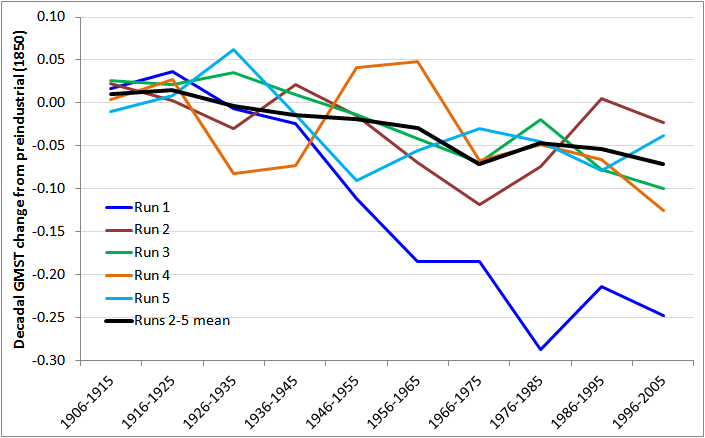
Figure 5: GMST responses to land-use change (LU) single-forcing runs
Although Marvel et al. do not mention the very low efficacy of solar forcing in their simulations, this appears to have more effect on ERF efficacy for the sum of forcings over the historical period than does low volcanic efficacy. The efficacy of solar iRF in four non-GISS CMIP5 models has been found to be much higher than in Marvel et al.’s simulations, varying between 0.72 and 0.85.[24]
Efficacy estimates from the Historical simulation
This is the most relevant case for comparison with observational estimates, as the effect of individual forcings cannot be observed in the latter. Comparisons based on iRF data are not very relevant since observational studies do not normally use iRF. The ERF data is in principle relevant, but some of the GISS-E2-R values are difficult to believe. The GHG ERF forcing change from 1850 to 2000 is 47% higher than the corresponding change per the best estimate in AR5.[25] After allowing for F2xCO2 being 4.1 W/m2 for ERF in GISS-E2-R rather than 3.71 W/m2 in AR5, 1850–2000 GHG ERF forcing is 33% higher relative to F2xCO2 in GISS-E2-R than per AR5, despite CO2 forcing making up more than half of GHG forcing (per AR5).
This extraordinarily large difference suggests both that F2xCO2 using ERF is well above 4.1 W/m2 in GISS-E2-R, and that in that model non-CO2 GHGs produce a far higher ERF relative to CO2 than per AR5 estimates. Using a regression-based ERF F2xCO2 of 4.5 W/m2,19 TCR estimated using the Historical simulations ERF data is 1.33°C, only 5% below GISS-E2-R’s TCR of 1.4°C. And with ΔQ divided by 0.86 to better approximate ΔN, the ECS estimate is 2.02°C, in line with GISS-E2-R’s effective climate sensitivity of 1.9–2.0°C. These comparisons shows the efficacy of Historical ERF to be very close to one. Interestingly, the same is true when Historical iRF is used, provided that the iRF F2xCO2 that Hansen 2005 found for ModelE, of 4.52 W/m2, is used. In the latter case, it becomes very clear that the outlier is the WMGHG response, which has an inexplicably high efficacy. When zero-intercept regressions are used for estimation, the transient efficacy of Historical iRF is then 1.02, and the equilibrium efficacy is also 1.02 (1.09 with ΔQ divided by 0.86), based on an effective climate sensitivity of 2.0°C for the model.
Marvel et al.’s critique of observational TCR and ECS estimates from particular studies
Marvel et al. calculate TCR and ECS estimates using forcing values from Shindell 2014, Otto et al. 2013 and Lewis and Curry 2014, both with and without adjusting the efficacies of each constituent individual forcing estimate used by each. This is a pointless exercise for iRF efficacies, since none of the studies use iRF values. And it is misleading for ERF, given that several of the single forcing efficacy estimates seem very questionable. Moreover, many of the calculated TCR and ECS best estimates (medians) in their SI Table 3 do not agree to the data from their SI Tables 1 and 2.[26]
It is also the case that even had Marvel et al.’s efficacy estimates and calculations been valid, they would have had no material implications for the Otto et al 2013 TCR and ECR estimates. That is because the underlying forcing estimates used in that study already reflect efficacies, contrary to what Marvel et al. imply.
Estimates based on recent observations can only be of effective, not equilibrium, climate sensitivity, since the climate system has not reached equilibrium. It is unknown whether the two values differ to any extent in the real world. They do so in many coupled GCMs; in GISS-E2-R the effective climate sensitivity relevant to Historical forcing is ~85% of the equilibrium value. But this has nothing whatsoever to do with forcing efficacies.
Conclusions
I have highlighted many serious problems with the Marvel et al. study. Because of them, its results would be of little or no relevance to observational estimation of TCR and ECS even if the real climate system responded to forcings similarly to GISS-E2-R. Using better justified estimation methods, and the GISS-E2-R effective rather than equilibrium climate sensitivity, the Historical iRF and ERF data are both found to produce efficacies within ~10% of unity, both using Marvel et al.’s estimates of the forcing from a doubling of CO2 and with them adjusted up. Marvel et al.’s claim to have shown that TCR and ECS estimated from recent observations will be biased low is wrong. Their study lacks credibility.
Appendix A: Further information about Hansen 2005 and other efficacy-related studies
Figure A1, which reproduces Figure 25(b) of Hansen 2005, summarizes its findings for Fs. The unmarked purple range with a best estimate (open circle) of 0.9 is for ozone. When aerosol indirect effects on cloud cover were included, tropospheric (anthropogenic) aerosol efficacy reduced from 1.14 to 0.99. These efficacy estimates take into account that some forcings (e.g. aerosols, ozone and land-use change) are spatially inhomogeneous. The efficacies relate to the response 100 years after a forcing was applied. This is a longer timescale than for TCR, where the weighted mean time from forcing being imposed to measuring the response is 35 years, but it is much too short to approximate the equilibrium response.
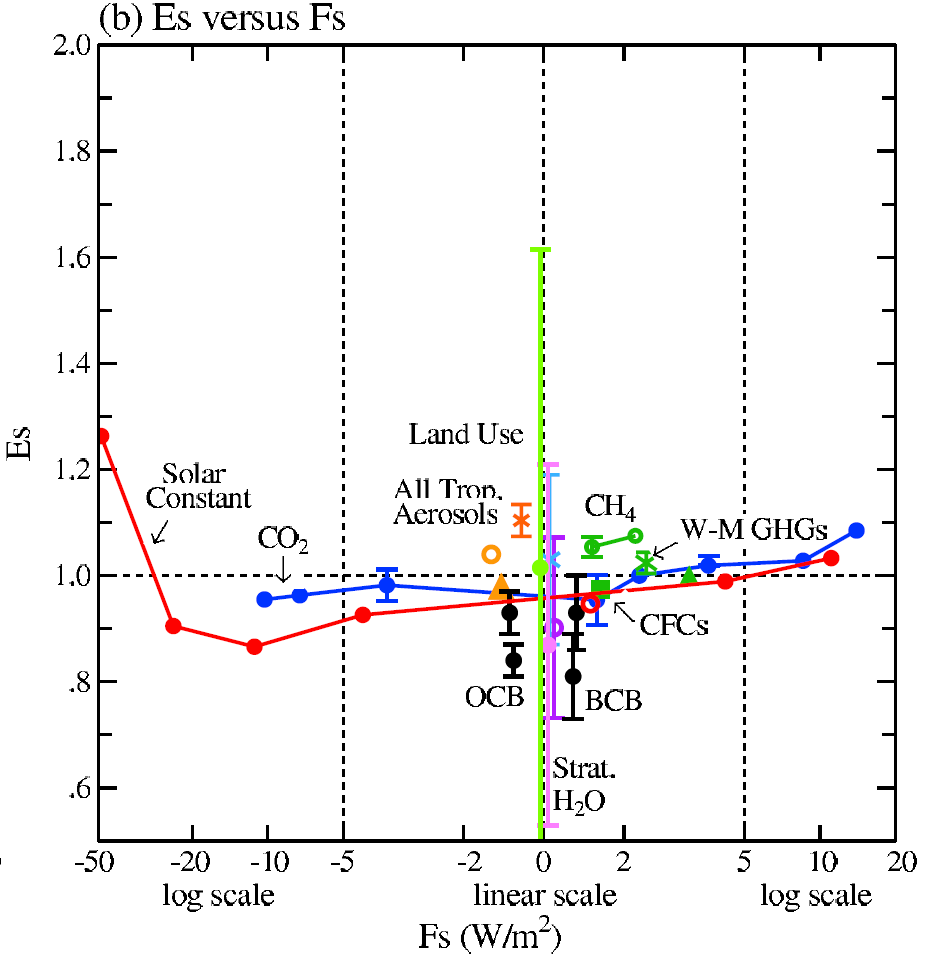 Figure A1. Reproduction of Fig. 25(b) Hansen et al (2005): Forcing efficacy relative to Fs (~ERF)
Hansen 2005 also estimated the efficacy for the sum of all the simulated transient responses to individual historical forcing changes, and for the transient response to all these forcings being applied at once. Using Fs, both efficacies were almost exactly one. This suggests that the transient responses to differing types of forcing are very comparable when forcing is taken as Fs. Hansen 2005 concluded that, at least for climate forcing agents over the historical period, Fs was a good measure of the effective forcing (the product of a forcing, however defined, and the efficacy taken relative thereto), notwithstanding that some forcings had different spatial distributions from others. However, the effect of soot (black carbon) deposited on snow and ice (SnowAlbedo_BC) was poorly constrained.
Another 2005 study,[27] which used a different model, also found that all efficacies were largely independent of the type of forcing, provided its measure accounted for tropospheric as well as stratospheric adjustment. Although the Hansen 2005 results were based on the behaviour of a single GCM, they were generally supported in AR5, which concluded that ERF is a better measure than RF of the eventual GMST response, especially for aerosols, although in most cases the difference was small. SnowAlbedo_BC forcing was, exceptionally, estimated to cause a two to four times larger GMST change relative to its RF than does CO2.
Subsequent to AR5, another NASA GISS scientist, Drew Shindell, published a study (Shindell 2014)[28] claiming that the transient response to spatially inhomogeneous forcings was significantly greater than that to GHGs, with the consequence that estimates of TCR based on comparing GMST and total forcing changes since circa 1850 were biased down. The dominant spatially inhomogeneous forcing is that from aerosols, but ozone and, to a minor extent, land-use change also contribute. Shindell’s study was based on comparing historical simulations with all forcings, GHG-only and natural-only forcings included. This is a less clean approach than using single-forcing simulations. It requires making various difficult-to-assess assumptions and adjustments, and magnifies the noise from model internal variability.
I find Shindell’s results difficult to reconcile with the observed evolution of hemispherical and tropical temperatures relative to GMST over the historical period. Moreover, they are contradicted not only by Hansen’s 2005 study, but also (in respect of aerosols) by the only other relevant published single forcing simulation based study [29] that I know of apart from Marvel et al. I am also aware of as yet unpublished work using another, state-of-the-art, GCM that likewise shows no evidence of a greater transient response to aerosol forcing than to CO2.
For completeness, I will add that following Shindell’s study, Kummer and Dessler published a paper[30] applying Shindell’s finding, that the efficacy of aerosol and ozone forcing was about 1.5, to the estimation of ECS, thereby obtaining a central value for ECS of over 3°C. Clearly, if Shindell’s findings are invalid, so are Kummer and Dessler’s.
Appendix B: Discussion of discrepancies in Marvel et al.’s ERF based TCR and ECS estimates
Marvel et al. state, in their Figure 1 legends, TCR and ECS estimates for GISS-E2-R implied for ERF basis forcings by the ΔT and ΔF−ΔQ values. The ECS values should be compared with the model’s effective climate sensitivity of 1.9–2.0°C. A comparison of the stated values with those calculated from the ΔT, ΔF and ΔQ data and from digitised values for ΔF−ΔQ is given in Table 3. Marvel et al.’s values almost all disagree, by varying ratios, with either of those I calculate. The last row of each section of Table 3 shows what the TCR and ECS estimates calculated from data revised as indicated would be.
Table 3: Marvel et al.’s ERF-based TCR and ECS estimates and recalculated equivalents
| Forcing agent/ Type & source of sensitivity | Aerosol AA |
Greenhouse gases GHG | Land-use change LU | Ozone Oz |
Solar SI |
Volcanoes VI |
Historical |
| TCR: per Fig.1a ΔF | 1.36 | 1.32 | 3.13 | 0.88 | 0.58 | 0.75 | 1.17 |
| TCR: stated in Fig.1a | 1.3 | 1.2 | 2.8 | 0.8 | 0.5 | 0.7 | 1.1 |
| TCR: on unadjusted data | 1.35 | 1.33 | 3.65 | 0.97 | 0.52 | 0.82 | 1.21 |
| With F2xCO2 revised | 1.49 | 1.46 | 4.00 | 1.06 | 0.57 | 0.90 | 1.33 |
| ECS: per Fig.1b ΔF−ΔQ | 2.14 | 1.90 | 2.54 | 1.28 | 0.58 | 1.12 | 1.64 |
| ECS: stated in Fig.1b | 2.0 | 1.7 | 2.4 | 1.2 | 0.5 | 1.0 | 1.5 |
| ECS: on unadjusted data | 2.08 | 1.90 | 3.04 | 1.46 | 0.54 | 1.32 | 1.72 |
| ΔQ/0.86; F2xCO2 revised | 2.50 | 2.25 | 3.25 | 1.75 | 0.60 | 1.61 | 2.02 |
Whatever the ERF F2xCO2 value used in Marvel et al. is, for every forcing agent the ratio of the ERF-based TCR stated in its Figure 1a to the ERF transient efficacy given in its SI Table 1 should equal the GISS-E2-R TCR of 1.4°C, and the ratio of the ERF ECS stated in their Figure 1b to the ERF equilibrium efficacy given in their SI Table 1 should equal the GISS-E2-R ECS of 2.3°C. However, save for solar forcing, the ratios calculated from the data imply a model TCR of 1.51–1.57°C, ~10% higher than its 1.4°C TCR. For ECS, omitting the obviously incorrect LU efficacy, all the ratios imply model ECS values in the range 2.11–2.15°C, nearly 10% lower than its 2.3°C ECS, again save for solar, which is further adrift.
[1] Kate Marvel, Gavin A. Schmidt, Ron L. Miller and Larissa S. Nazarenko, et al.: Implications for climate sensitivity from the response to individual forcings. Nature Climate Change DOI: 10.1038/NCLIMATE2888. The paper is pay-walled, but the Supplementary Information (SI) is not.
[2] The Historical simulations have an average temperature anomaly of 0.84°C for 1996–2005 relative to 1850, whereas HadCRUT4v4 shows an increase of 0.73°C from 1850–1859 to 1996–2005, and Figure 7 of Miller et al. 2014 shows consistently greater warming for GISS-E2-R than per GISTEMP since 2000. The same simulations show average ocean heat uptake of 0.84 W/m2 over 1996–2005 (mean slope estimate), compared to 0.40 W/m2 using AR5 Box 3.1, Figure 1 data, or 0.67 W/m2 using NOAA (Levitus et al. 2012) data.
[3] Hansen J et al (2005) Efficacy of climate forcings. J Geophys Res, 110: D18104, doi:101029/2005JD005776
[4] Chapter 8 of AR5 is available here.
[5] See Section 10.8.1 in Chapter 10 of AR5 for a discussion of the use of these equations in estimating TCR and ECS.
[6] Miller, R. L. et al. CMIP5 historical simulations (1850_2012) with GISS ModelE2. J. Adv. Model. Earth Syst. 6, 441_477 (2014).
[7] Or with climate state, but feedbacks vary little with climate state, within limits, in most GCMs.
[8] I estimate GISS-E2-R’s effective climate sensitivity applicable to the historical period as 1.9°C and its ERF F2xCO2 as 4.5 Wm−2, implying a climate feedback parameter of 2.37 Wm−2 K−1, based on a standard Gregory plot regression of (ΔF − ΔN) on ΔT for 35 years following an abrupt quadrupling of CO2 concentration. The efficacy-weighted mean period from the imposition of incremental forcing to the end of the historical period is of this order. I also estimate the model’s effective climate sensitivity, as 2.0°C, from regressing the same variables over the first 100 years of its 1% p.a. CO2 increase simulation; this estimate is little affected by F2xCO2 value.
[9] Miller et al. 2014 noted a 15% increase in GHG forcing in GISS ModelE2 compared to the CMIP3 version ModelE, despite their forcing (RF) for a doubling of CO2 being nearly identical, but were unable to identify the cause.
[10] The 0.86 divisor comes from the coefficient on the integral of TOA imbalance anomaly ΔN when regressing the ocean heat content (OHC) anomaly against both that integral and time, thus isolating any fixed offset between ΔQ and ΔN that may exist.
[11] The 1996-2005 ΔT for the sum of the six single-forcing cases is 0.76°C, compared to 0.84°C for Historical (all forcings). For iRF, the corresponding ΔF values from the archived data are 2.53 W/m2 and 2.75 W/m2. However, the values plotted are 2.74 W/m2 and 3.05 W/m2 respectively. For ERF, the sum-of single forcings and the Historical forcing ΔF values from the data are respectively 2.99 W/m2 and 2.84 W/m2, but the values plotted in Figure 1c are 3.03 W/m2 and 2.93 W/m2.
[12] Otto et al. used regression-based estimates of ERF in multiple CMIP5 models. Lewis and Curry used estimates from Table AII.1.2 of AR5, which are stated to be ERFs but in most cases (aerosol forcing being the most notable exception) assessed to be the same as their RFs.
[13] The AR5 Glossary (Annex III) states: ”The traditional radiative forcing is computed with all tropospheric properties held fixed at their unperturbed values, and after allowing for stratospheric temperatures, if perturbed, to readjust to radiative-dynamical equilibrium. Radiative forcing is called instantaneous if no change in stratospheric temperature is accounted for.” And early in Chapter 8 it says: ”RF is hereafter taken to mean the stratospherically adjusted RF.”
[14] However, Hansen 2005 found that only in the cases of aerosol and BCsnow forcing was there a major difference between RF and ERF. AR5, after surveying a wider range of evidence, reached similar conclusions, and accordingly in other cases estimated ERF to be the same as RF, with an implied efficacy estimate of one, but gave wider ranges for ERF to allow for uncertainty in the relationship between ERF and RF.
[15] AR5 states (Section 7.5.1 of Chapter 7): ”it is inherently difficult to separate RFaci from subsequent rapid cloud adjustments either in observations or model calculations… For this reason estimates of RFaci are of limited interest and are not assessed in this report.”
[16] Transient efficacy estimates using iRF based respectively on unconstrained decadal regression from 1906–2015 to 1996–2005 (as in Marvel et al.), changes from 1850 to 1996–2005, and zero-intercept regression are: LU 3.89, 1.64, 1.03; Oz 0.60, 0.57, 0.70; SI 1.53, 1.68, 1.82; and VI 0.56, 26.45, 0.31. In principle, using changes is preferable to zero-intercept regression for transient estimation because of the ‘cold start’ issue, but its superior noise suppression leads to more consistent estimation from zero-intercept regression when forcing is small.
[17] Schmidt, G. A., et al. (2014): Configuration and assessment of the GISS ModelE2 contributions to the CMIP5 archive, J. Adv. Model. Earth Syst., 6, 141–184, doi:10.1002/2013MS000265.
[18] The GHG forcing in 1996–2005 is 10% higher in ERF than in iRF terms. GHG forcing in 1996–2005 was dominated by CO2, and Hansen 2005 found GHG had an efficacy of very close to one both in terms of Fs, which is very similar to ERF, and using iRF (1.02 and 1.04 respectively). That suggests scaling the actual F2xCO2 iRF of 4.1 W/m2 by the ratio of Marvel et al.’s iRF and ERF values for GHG forcing, which implies a 10% higher F2xCO2 ERF, of 4.52 W/m2. That value is also in line with F2xCO2 of 4.53 W/m2 estimated from a Gregory-plot regression over the 35 years following an abrupt quadrupling of CO2.
[19] There were no material differences between the digitised and data values for ΔT, so I used only the data values, which were more precise. Note that Marvel et al. do not specify whether, for ERF efficacy estimates, ensemble means are taken before or after calculating quotients. As only a single forcing value is given, and ensmble means were taken before regressing in the iRF case, I have assumed the former, which also seems more appropriate.
[20] Lewis N, Curry JA (2014) The implications for climate sensitivity of AR5 forcing and heat uptake estimates. Clim. Dyn. DOI 10.1007/s00382-014-2342-y. Non-typeset version available here.
[21] Shindell, D. T., et al., 2013: Interactive ozone and methane chemistry in GISS-E2 historical and future climate simulations. Atmos. Chem. Phys., 13, 2653–2689. This study found that iRF ozone forcing from 1850 to 2000.was 0.28 W/m2 when the climate state was allowed to evolve in line with the Historical simulation and 0.22 W/m2 when a fixed present-day climate was used, and ERF was calculated as 0.22 W/m2. These values are substantially below those used in Marvel et al. of 0.45 W/m2 iRF and 0.38 W/m2 ERF. Substituting Shindell et al.’s values for Marvel et al.’s would raise the ozone iRF and ERF transient efficacies values to respectively 0.92 and 1.18.
[22] If one excludes LU run 1, no individual run for any forcing (including Historical) produces a 1950-2005 mean GMST response that differs by more than 0.031°C from the ensemble mean response for that forcing. But for LU run 1 the difference is -0.134°C (and would be -0.168°C were run 1 excluded from the ensemble mean).
[23] Chapter 8 of AR5, referring to a seven model study, states that ”There is no agreement on the sign of the temperature change induced by anthropogenic land-use change” and concludes that a net cooling of the surface – accounting for processes that are not limited to the albedo—is about as likely as not”.
[24] Schmidt H et al. (2012) Solar irradiance reduction to counteract radiative forcing from a quadrupling of CO2: climate responses simulated by four earth system models Earth Syst. Dynam., 3, 63–78
[25] The GISS-E2-R increase in GHG ERF is 3.39 W/m2. The 1850-2000 increase in GHG RF and ERF per AR5 Table AII.1.2 is 2.25 W/m2, but I use the higher 1842–2000 increase of 2.30 W/m2 since the 1850 CO2 concentration in GISS ModelE2 was first reached in ~1842, according to the AR5 data.
[26] I calculate TCR and ECS values as shown in the below table, from the efficacies stated in Marvel et al.’s SI Table 1 (digitising from their Figure 1 for GHG). [E=1 means assuming all efficacies are one.]
| Median estimates | Shindell 2014 | Lewis and Curry 2014 | Otto et al 2013 | |||||||
| E=1 | iRF | ERF | E=1 | iRF | ERF | E=1 | iRF | ERF | ||
| TCR | ||||||||||
| As stated in SI Table 3 | 1.4 | 2.0 | 1.9 | 1.3 | 1.6 | 1.7 | 1.3 | 1.8 | 1.8 | |
| From SI Table 1 (GHG from Fig.1) | 1.98 | 1.58 | 1.92 | 1.60 | 1.92 | 1.69 | ||||
| ECS | ||||||||||
| As stated in SI Table 3 | 2.1 | 4.0 | 3.6 | 1.5 | 2.0 | 2.3 | 2.0 | 2.9 | 3.4 | |
| From SI Table 1 (GHG from Fig.1) | 3.88 | 3.48 | 2.77 | 2.73 | 3.90 | 3.78 | ||||
[27] Sokolov, A P (2005): Does model sensitivity to changes in CO2 provide a measure of sensitivity to other forcings? J Climate, 19, 3294-3305
[28] Shindell, DT (2014) Inhomogeneous forcing and transient climate sensitivity. Nature Clim Chg: DOI: 10.1038/NCLIMATE2136
[29] Ocko IB, V Ramaswamy and Y Ming (2014) Contrasting climate responses to the scattering and absorbing features of anthropogenic aerosol forcings. J. Climate, 27, 5329–5345.
[30] Kummer J. R. and A. E. Dessler (2014): The impact of forcing efficacy on the equilibrium climate sensitivity. GRL, 10.1002/2014GL060046
Update: Data and calculations are available here, in Excel form


83 Comments
“The efficacy of a forcing is defined as its effect on GMST relative to that of the same amount of forcing by CO2.”
Notwithstanding those who like to count joules in the deep oceans, if that definition is reasonable then what does it say about whether the feedbacks should have (un)equal efficacies? In other words, if forcings are not all equal, then it seems reasonable to ask if feedbacks are not equal either.
Nic, thanks for this impressive discussion.
Why did they stop in 2005? Is that the last year/common year in Otto et al (2013), Lewis and Curry (2014), and Shindell (2014)?
No, it is not. Cherrypick?
In your introduction, if you change ‘assert’ to ‘contend’ it would make the beginning of your paper sound less a bit less charged.
What’s remarkable about your piece here is the clarity of the English writing. I was able to follow it all despite being a non-scientist.
Thanks for the hard work. My only other suggestion would be a quick section on how you would recommend Marvel et al proceed to improve their work.
thomasfuller2, thanks for your comment.
There was no intention on my part to use a charged term. I consider “assert” to be a more neutral term than “contend”. See http://the-difference-between.com/contend/assert
“the difference between assert and contend is that assert is to declare with assurance or plainly and strongly; to state positively while contend is to strive in opposition; to contest; to dispute; to vie; to quarrel; to fight.”
Marvel et al could withdraw their paper and submit a new one, using more satisfactory methodology and providing more detail, after performing a set of simulations that showed how the GISS model responded to each type of forcing as the climate state evolved during the historical period. Preferably extended to 2012, to match the simulation results in Miller et al 2014 (which is a much higher quality paper). But I see very little chance of that happening.
There is in any case a question mark over how suitable a model GISS-E2 is for this purpose. As I indicate in the article, GISS-E2 seems to have amazingly high forcing from non-CO2 long lived greenhouse gases (methane, nitrous oxide, CFCs etc), and a remarkably strong GMST response to them, if the forcing from a doubling of CO2 in the model is as taken in Marvel at al.
Couple of questions on the last para:
1. Which GCM would in your view have been better? How easy is that to even evaluate?
2. How long (elapsed) would it have taken to run the various simulations for the different forcings on GISS-E2, leading to the write-up in Marvel et al? On the standard GISS supercomputer, under standard loading, or whatever they would have had available?
I realise it may only be the authors who can give any idea of the second but it would be interesting to get a feel for how easy it would be for others to play around with this stuff. I’m still, after six years, struggling with what openness if climate software even means, compared to areas with which I’m much more familar.
RichardDrake,
1. Probably best to use a number of unconnected AOGCMs from different groups. Perhaps focussing on those from grous in western Europe and North America, judging from the views of the modellers I have met.
2. I suspect a fair while. See my response to Alberto Zaragoza Comendador, below.
Nic, “GISS-E2 seems to have amazingly high forcing from non-CO2 long lived greenhouse gases (methane,” Very interesting since Gavin discourages ppl from worrying about methane & even got into a row w/ Wadhoms (sp) over it… How different are their scenarios? I assume very different?
Sue, As I say in note 25: “The GISS-E2-R increase in GHG ERF is 3.39 W/m2. The 1850-2000 increase in GHG RF and ERF per AR5 Table AII.1.2 is 2.25 W/m2, but I use the higher 1842–2000 increase of 2.30 W/m2 since the 1850 CO2 concentration in GISS ModelE2 was first reached in ~1842”. If one strips out the CO2 contributions, of 1.38 W/m2 for AR5 (based on an F2xCO2 of 3.71 W/m2) and of ~1.53 W/m2 for GISS-E2-R (based on an ERF F2xCO2 of 4.1 W/m2) the the contribution of the other long lived GHG is 0.92 W/m2 per AR5 and ~1.86 W/m2 for GISS-E2-R.
That is, methane, nitrous oxide, CFCs and minor GHGs add TWICE as much forcing in GISS-E2-R as per the AR5 best estimate.
As I wrote, it looks as if GISS-E2-R radiative transfer computation in GISS-E2 may be inaccurate.
Although methane is classed as a long-lived GHG, its lifetime is only of the order of a decade, so it presents much less of a long term problem than CO2, part of which is expected to remain in the atmosphere for 1000+ years. On the other hand, as well as being a powerful GHG it is a source of tropospheric ozone and stratospheric water vapour, both of which add to the basic forcing from methane.
niclewis:
Another interesting feature of methane is when it breaks down, it (largely?) breaks down into C02. There is far less methane in the atmosphere than C02, but that effect may well have contributed a couple percent to the observed rise in C02 levels.
There is no reason to believe that excess CO2 will remain in the atmosphere very long. Already only about half of the human produced CO2 in any given year (as can be calculated from the atmospheric CO2 increase). The other half is immediately removed by nature. This indicates that a 33% increase in CO2 causes the natural removal processes to increase by this amount. Therefore, if we stopped all emissions, we should cause CO2 to decline at about the same rate as it now is increasing. This is so, because the increased absorption persists until CO2 is lower. At that rate, it would not take thousands of years to remove all the CO2 from fossil fuels, but less than one hundred years. (This timescale is also in agreement with the rapid decline of the C14 spike due to atmospheric nuclear explosions in the fifties.)
Nic: “This definition is reasonable: CO2 is the dominant greenhouse gas”
###
Next to water vapor, you must mean.
GHG here means long-lived greenhouse gases, which excludes ozone as well as water vapour. But I am afraid the definition appears after the term GHG has already been used.
Thank you, Nic, for yet another detailed study.
There is a matter arising from observations about relations between land temperature and local rainfall. For example, at several Australian weather stations studied in detail with statistics, recorder local rainfall correlates with recorded temperatures quite significantly. That is, GHG are not the only driver of temperature changes as recorded. Wetter is cooler. Rainfall does not seem to sit within the 7 individual forcings you have studied (it might, pls correct if I am wrong). Given that local rainfall statistically can account for 30-50% of the variation in local temperatures and given that simple physics help explain this, I am left wondering where the effect of rainfall on local temperatures in inserted into sensitivity studies, if indeed it needs to be.
As studies become more detailed, it is likely that many odd questions of this type will emerge. Another is from the Dec 2015 Schmidtusen GRL paper claiming a cooling over the Antarctic as atmospheric CO2 increases. IR emissions to space do not come from the ground surface there because it is too cold, so the use of land surface as a reference layer elsewhere might be compromised. While models might gather up local effects like these, they can be hard to track down. Even if they are incorporated, one wonders if the mathematics in the models are set to sum or integrate only positive values of sensitivities at defined locations (not ECS or TCR as globally defined, but locally).
I hope I am not wasting your time here. There are bigger problems for us at home, preventing some detailed digging.
Thanks, Geoff. Forcings generally have (in GCMs) similar global effects, even if they are concentrated in particular regions or differ between the hemispheres. Figure 24 of the Hansen 2005 paper that I provided a link to shows this very well. But variation in local feedbacks (and hence in local climate sensitivity) does seem to have more local effects. GCMs do incorporate this, although their simulations of feedbacks and their effects may not be correct. The models don’t distinguish between positive and negative local sensitivities. In many GCMs, sensitivity is negative in the deep tropics: net outgoing radiation goes down when surface temperature increases, because water vapour and cloud feedbacks are so strongly positive there. That means there would be runaway warming there if heat from the deep tropics couldn’t be exported to higher latitudes. Maybe not hte sort of ‘negative’ sensitivity you had in mind, but it proves the point.
Models generally aren’t very good at simulating changes in rainfall patterns to increasing GHG and resulting global warming. But they do all agree that total rainfall will increase. In fact, the lower climate sensitivity is, the faster must total precipitation increase with GMST, or the atmosphere would heat up too much. But where the extra rain falls is a different question – it could almost all be over the oceans.
Does that mean that recent flooding in the UK is evidence for low climate sensitivity. 😉
Got there before me Bish! But this last paragraph plugged an important gap in my understanding, thank you Nic. There may be others 🙂
I asked Gavin Schmidt´s comment on your review on his co-article on Realclimate and he answered: “Mostly confused, but there are a couple of points worth following up on. Should have the relevant sensitivity tests available next week. – gavin]”
http://www.realclimate.org/index.php/archives/2016/01/marvel-et-al-2015-part-2-media-responses/#comment-640742
+1 Looking forward to his follow up…
” 1.00 for CO2 forcing”
C’mon. Water is what? 1.9? The feedbacks are entirely hypothetical. The radiative forcing of CO2 is expressed as unity, entirely ignoring its “saturation”.
While the trends of temperature and Co2 are mysteriously different, the variability of CO2 is substantially captured by temperature, even in the last 35 years.
Gymnosperm,
As intensively discussed here:
Most of the variability of the CO2 rate of change is caused by the influence of temperature variability (Pinatubo, El Niño) on (tropical) variation. That is proven by the opposite CO2 and δ13C changes:
Vegetation is not the cause of the trend in CO2: it is an increasing sink for CO2, at least since 1990:
http://www.sciencemag.org/content/287/5462/2467.short
and
Click to access BenderGBC2005.pdf
Variability and trend of CO2 have nothing in common, they are driven by different processes…
It would seem that their methodology (single-forcing model runs) would be most valuable in identifying areas for improvement in the GISS-E2-R model. I am at a loss to see how that methodology would be superior to estimating TCR/ECS directly from observational data sets.
Perhaps the answer lies behind the Marvel, et al., paywall but did they calculate the relative contribution from each single-forcing estimate to the ultimate increase in their respective TCR/ECS estimates?
Observational based studies must make some estimate of the forcing which gave rise to the observed temperature. If a large forcing is assumed/estimated then this implies a low climate sensitivity. Conversely a low forcing giving rise to the same observed temperature gain implies a high climate sensitivity.
By definition TCR and ECS relate only to CO2 forcing. It is known that, in the models at least, not all forcings produce identical temperature responses – some higher than expected from a CO2 equivalent forcing and some lower than expected. Marvel et al argue that by “an accident of history” the apparent summed forcings are higher than they would be if all of the forcings were expressed in terms of their equivalence to CO2 forcings. By so doing they argue that the total forcings used as input into observational studies are too high (relative to CO2 equivalence) and hence climate sensitivities (which again have to be CO2 specific) are therefore biased low.
Hope this helps.
opluso
Their work certainly highlights some peculiarities in the GISS model.
Your question is a good one. Marvel don’t give any results for the relative contributions of diferent forcings to their increases in observational TCR/ECS estimates. I have worked them out for TCR using ERF forcings; this is the only case for which their methodology doesn’t need changing; the true ERF F2xCO2 value is unknown but varying it would change all contributions in the same direction.
Their very high efficacy for land-use is the biggest contributor, closely followed by the slightly sub-unity efficacy of GHG, and then by the pretty low efficacy for ozone (broadly, half as important as LU). Aerosols and solar have similarly small but opposing effects. Volcanic should be small, but I think they’ve got the wrong VI forcing for the Otto and Shindell studies – they made their own estimates of this forcing, I believe.
Nic,
Thank you for the detailed and thoughtful input to this problem.
Before making a comment on the results, I would like to underline that, outwith the gross methodological errors in Marvel et al, there are two elements which I find bizarre.
Firstly, to do efficacy comparisons meaningfully requires carrying at least 3sf accuracy through the calculations of derivative data. One piece of fundamental input is the evolution of net flux, or, at a minimum, an accurate estimate of the change in net flux over a pre-specified period. In this context, Marvel’s choice of using OHC data rather than making direct use of the available net flux data from the model runs seems absurd. In observation-based estimates of CS and feedbacks, researchers are forced to use OHC data as a means of accessing net flux estimates over the longer term. This requires some fairly coarse assumptions to be made, including what percentage of any net flux imbalance is converted to sensible heat in the ocean (as you point out). Going from model-calculated OHC back to net flux imbalance in the model with any accuracy is extremely difficult, since as well as the “natural” net flux variation in the pre-industrial control which is integrated in some guise into the GCM’s energy accumulation and needs to be discounted, there is also conversion of radiative input into sensible heat and latent heat, conversion to momentum flux and distribution of sensible heat between land, sea and atmosphere. In addition, there is energy leakage from the model climate system; it is not fully conserved. All of these elements are model-specific. I can quite honestly think of no excuse for the use of OHC data in this context, when the net flux data should be available to the GISS researchers. Its sole consequence in the efficacy calculations is the introduction of unnecessary error and uncertainty.
Secondly, engineers would recognise an efficacy calculation as a “benchmark calibration” study. A fundamental requirement for such a study is to have the benchmark measurements available. Hansen 2005 recognised this and took great pains to measure the forcing data for the CO2 cases – which form the benchmark against which all other responses are calibrated. He provided estimates of Fi(iRF), Fa(RF) and Fs(ERF) across a range of concentrations of CO2. Commendable. For Marvel et al, on the other hand, we have a statement in Miller saying:
“However, forcing associated with a doubling of CO2 is nearly identical between the CMIP3 and CMIP5 models [Hansen et al., 2005; Schmidt et al., 2014a]”
This is then contradicted by the “iRF value” cited in Marvel et al and the Fa values in Schmidt 2014. No reference is provided at all for ERF values. This is a dog’s dinner – a benchmark study without benchmarks.
The above two elements strongly suggest to me that this did not start as an efficacy study. My speculation is that it started as a study to show that by applying the same methods used in observation studies to the GISS-ER-2 data, you got the wrong answer for sensitivity. They then found that you actually got very compatible answers if done with reasonable estimates of historical forcing and a sensible treatment of OHC. The study then morphed into one which had to show that the historical forcing had an overall weighted average efficacy less than unity. I can think of no other explanation for carrying out an efficacy study which uses OHC instead of net flux and which is based on a woefully inadequate definition of the benchmark data on the CO2 cases.
kribaez,
The paper is clearly an effort to discount the lower sensitivity estimates from empirical studies; how the Marvel et al work evolved is speculative, but the overall objective is obvious: discount all (low) empirical estimates of TCR and ECS.
There have been several other papers from GISS where GCM behavior was used to discount lower empirical estimates of sensitivity; one paper critical Stephen Schwartz’s temperature autocorrelation based estimate of sensitivity immediately comes to mind. The general class of paper can be described as “you can’t ever show the GCM projections are too high by using actual data.” In other fields, efforts to discredit empirical data rather than improve a model would be laughed at, but is, oddly enough, taken very seriously in climate science.
I will go out on a limb and predict GISS will produce similar critiques of other empirical estimates in the future.
Yes, the rebuttal to Schwartz is a very pertinent analogue. In that instance, the GISS team argued that the Schwartz method could not be sound because when applied to GISS data it gave the wrong answer for climate sensitivity. The reality was that it actually gave the correct answer for GISS climate sensitivity over the temperature interval tested. The error in the rebuttal was the failure to recognise the difference between the effective equilibrium temperature and the model-reported ECS. Because of the curvature in the net flux vs temperature relationship for a step-forcing which GISS exhibits (like most GCMs), the latter is not tested. The identical error (among others) is being made in the Marvel et al study.
And of course Giss have the unique advantage of adjusting their own empirical data to fit what their model predicts. For a while the satellite data was a minor constraint on doing that but since ‘Best’ (sic) avoided reconciling satellite data (with a sideways swipe) it seems Giss felt ok to follow suit. The next step will be twisting Carl Mears arm to apply an upwards adjustment to RSS and leave UAH as the lone outlier run by easily dismissible skeptics. It all plays like a handbook of how to distort research in support of a predetermined agenda.
kribaez,
Thank you for your comment. I compltely agree with you about the use of OHC rather than TOA radiative imbalance data, and the lack of benchmark values for the forcing from a doubling of CO2.
Using the OHC slope rather than TOA radiative imbalance N seems bizarre, and scientifically indefensible. It does, of course, produce biased-low estimates of the model ECS from historical period forcings – or indeed from any type of forcing.
Schmidt 2014 states GISS-E2-R has a stratospherically-adjusted (Fa) F2xCO2 value of 4.1 W/m2, which is in line with the 4.08-4.12 W/m2 for Fa in GISS-E per Hansen 2005. But Hansen gives the iRF (Fi) value as 4.52 W/m2, whereas Marvel uses 4.1 W/m2.
Nic,
Thanks for this clearly written post. Two questions:
1) Since you were a coauthor of two of the three empirical estimate papers (which Marvel et al claim to be inaccurate), it seems to me that the journal editor should have considered you as a reviewer. Were you asked to review the paper?
2) Are you and/or others considering submitting a comment on Marvel et al to the journal?
stevefitzpatrick,
Thanks. I answer to your questions:
1) No, I wasn’t
2) I shall reserve my position on that, but I am aware that journals often seek to avoid publishing comments. I suspect Nature CC may be worse than most in this regard. Comments also have very tight length restrictions.
IFAIK Nature ( not Nature CC ) has something very restrictive like 500 word limit (!) and a 6mo shut out.
500 words? No problem, give an abstract on each point and links to Climate Audit.
Marvel et al say near the end that ‘the historicalMisc archive is sparse’ and ‘these experiments were a low priority in CMIP5’, so ‘very few groups performed comparable calculations of radiative forcings associated with each forcing agent’. Yeah, I’m using the free version and cannot copy&paste. But their point is clear: replication will be difficult.
The thing is at least one paper mentioned by Nic, Ocko et al 2014 (reference 29), had done the same kind of experiments and arrived at different conclusions. But Marvel et al don’t cite Ocko either in the paper itself or in the SI.
My question to Nic would be: are these problems with historicalMisc (whatever that may be) real? Or is the lack of single-forcing experiments more due to plain lack of interest from researchers?
Non-paywalled version here:
http://www.nature.com/articles/nclimate2888.epdf?referrer_access_token=yt4E4zMaVXuZDScV8LGmN9RgN0jAjWel9jnR3ZoTv0MO1zBc6VqRZM1xVU1Fv4jKnwGY4K1Ah_7GxI9NoRjhKU_Hl2EiLRO5iCcrsnJkDxoEfAwgXzvzQK9VItUq66CXm98cMhK8Gyw5upFKumn8tA%3D%3D&tracking_referrer=realclimate.org
Good question. I’m not a modeller so I’m unsure of the answer. I suspect both are factors.
Working out forcings each year is computationally demanding, even when done for only one case and using iRF. MIller et al 2014 say, in relation to Historical vs Historical natural vs Historical anthropogenic “Computation of the total instantaneous forcing for each ensemble is expensive.”, and they only did it for GISS-E2-R NINT, not the other five GISS-E2 model variants.
But I also suspect that there has been some lack of interest by modellers in this area. Hopefully it will be better in CMIP6. There is also something called RFMIP that will focus on radiative forcings in models.
Quick excerpt from ATTP’s critique (link below) of this highly educational piece by Nic:
So now we know.
Thanks for that, I had to laugh.
It would seem more appropriate to cry.
It is amazing that an allegedly bright astronomer can spend so much time with his blog patrons essentially repeating again and again that their definition of the word audit is right and the dictionary definition is wrong. SteveM can take credit for giving the work audit a bad name among warmists. The other red herring seems to be that if its not peer reviewed, it can’t be right or at least it can be ignored if you believe it to be wrong even though you haven’t read it. 🙂
Given the level of effort involved in Marvel, et al., it is a bit disingenuous to argue it is merely a “critique” and not a full-blown audit of Otto, etc.
The purpose of Marvel, et al., was clearly revealed by co-author Schmidt at RealClimate. With an eye toward the next IPCC report, they wanted to stop the building momentum of observational studies that suggest lower climate sensitivities.
It was critique-good, audit-bad that amused me. The tear ducts sometimes fail from useruse.
Useruse sobs gonna be all night.
======
Nic, As always a very deep technical post and analysis. I personally am unqualified to wade through all the details given time restrictions. My question is whether it will ever be possible to get a technical debate on this topic either here or at Real Climate. I understand the history of the conflict between Schmidt and SteveM. But I would expect someone like Schmidt who is not directing a US Government institute to be willing to participate. This is an issue of job responsibilities and he should be able to put aside his personal feelings. I’m not sure I’m the one to do it but should someone send Schmidt an invitation to participate? The one thing that is clear is that Steve maintains very tight moderation constraints which could I think make this discussion productive and at least identify the points of disagreement.
I don’t understand your question. This is a technical debate. This is how it’s done. Schmidt or Marvel etc. may publish a rebuttal to this article, either in the comments here or elsewhere. Lewis may publish a rebuttal to that.
What do you want, that they should each have three minutes to comment? Do you see how much work went into this post? This way is better.
Nicholas, concludes: “Marvel et al.’s claim to have shown that TCR and ECS estimated from recent observations will be biased low is wrong. Their study lacks credibility.”
In my opinion, all those studies about TCR & ECS, (cited in this article), have no credit (including Lewis & Curry’s study).
The first big issue is about the accuracy of estimations: (a) there are discordant trends of present: low atmospheric satellite measured temperature vs. GST measured in land & oceans; (b) there is a big uncertainty linked to the proxy data obtained during XX, XIX and beyond centuries.
The second is about methodology: if we could proove that climate behaves in: a linear (or even in a cyclical) way, those TCR & ECS studies could make some sense: just as they are (or as a first approximation for small perturbations). But not such proof exists. Instead, what maths could we use in a better trustable way?.
Antonio, While it is true that there are large uncertainties in climate studies of sensitivity, some methods are more justified than others. This is true in my field of CFD as well. One thing that is certainly true is that energy is conserved in the climate system. If all the energy fluxes are accounted for in a reasonable way, there is some chance of getting the sensitivity in the ball park. We do this all the time with aerodynamic drag. Even though we have high uncertainty in CFD simulations in a lot of situations, sometimes simple models do work pretty well. Even though there are a lot of deep weeds in these things, they can work pretty well.
I do not think that Computational Fluid Dynamics is the appropriate way to understand climate sensitivity. Anyhow, I am courious about yourself, in what university did you learn about aerodynamic drag?.
Antonio, I work at a large aerospace company and have about 40 experience in these matters. GCM’s as Nick Stokes acknowledges are simply CFD solvers with complex sub grid models. In climate modeling, we are looking for a change in energy balance that is a couple of orders of magnitude smaller than the size of the overall energy fluxes so its very challenging. Aerodnamic drag is likewise 2 orders of magnitude smaller than the lift force so the computational challenges are similar. In CFD, we are a little bit more humble about our capabilities I think.
Humility: another sub-grid phenomenon, like thunderstorms.
I think that a great part of the ‘hostility’ towards the concept of climate sensitivity comes because it’s not a physical force or constant, like the gravitational constant, but the way people talk about it can make you believe that it’s treated as such. If you read an energy-budget estimate you will find:
-Sensitivity from 1870 to 2010
-From 1930 to 2010
-From 1870 to 2000
And so on. And the figures are slightly different, though the authors will recommend using the ‘best’ estimate (usually the one that covers the longest period and has the least natural noise, such as volcanic activity).
In other words, the temperature increase from a given radiative forcing (3.7w/m2 in the case of ‘standard’ sensitivity, i.e. a doubling of CO2) will be different depending on some other factors that are never ‘held constant’ and cannot be completely measured, so there isn’t a single sensitivity figure. Cloud cover changes, ocean currents change, vegetation changes, etc. Which means that the proportion of heat in the ocean as opposed to the atmosphere might be slightly different (big deal because the oceans store so much heat), that albedo might be slightly higher because you have less areas covered by forests which are darker than clear land and thus absorb more sunlight, and so on.
Of course the people who study this stuff try to account for changes in vegetation, for instance; that’s called land-use forcing. But guessing which changes in vegetation are natural and which are man-made is tricky to put it kindly.
As an amateur, in my opinion the biggest ‘known unknown’ is natural changes in cloud cover (and height and optical depth). Clouds are extremely complicated because they cause cooling (reflected sunlight) AND warming (greenhouse effect), and they react both to man-made and natural ‘forcings’. For example, an increase in forest area can lead to more tree-borne aerosols which in turn leads to more clouds.
One of the things I’ve wondered about is how can anyone derive ECS from paleo records. Even if you have a good estimate of temperatures, you then need an estimate of forcing, which has to include insolation. And even if you have a good estimate of insolation, you know nothing about what the clouds are doing. It would even be hard to know whether a change in insolation was caused by changes in the Earth’s tilt/orbit, i.e. Milankovitch forcing, or cloud changes. Even the greenhouse forcing will be inaccurate if you don’t know what clouds are doing.
TL; DR: ‘sensitivity’ is not a physical constant. But nobody is going to say ‘sensitivity from 18XX to 19XX’ every time he uses the concept, or ‘sensitivity assuming blahblahblah’; we simply talk about ‘sensitivity’, period. And that means people confuse it with the speed of light or similar constants.
Or to put it unkindly … OK, I won’t. Let’s just say Nic has done some herculean clearing of the undergrowth.
Alberto, I do agree that sensitivity is a complex concept and very context dependent. I also agree that its hard to understand how people can claim to derive accurate sensitivity estimates for the last glacial maximum for example, given the large uncertainties.
I look at it as establishing an upper bound rather than an accurate estimate.
Nic, good review and discussion here.
Is it appropriate for the Marvel authors to, or did they, attempt to put confidence intervals on their estimates of TCR and ECS using their methods?
Will this paper be discussed at Real Climate and if so would you be invited to participate?
Could you author and publish a paper using the approach in Marvel but with more appropriate methods and data?
I have a general question here that is OT but I thought I might best get a quick answer with this audience. I have been analyzing the Karl 2015 paper and the authors trend evaluations and in doing so as a side issue I wanted to compare my results on the New and Old Karl temperature series with CMIP% climate models. I am looking at the changes in 24 year trends with the following 15 year trends. In looking at the rate of change in warming I found what of which I was somewhat aware previously but still a little surprised to find the warming slow down over the periods just before and after the join year of 2005 where the Historical part of the RCP scenarios meets the scenario part of the series. What I find is the rate of warming (and forcing from a single source I have recently read) actually slows down for some period of time after 2005 depending on the RCP being 4.5, 6.0 or 8.5.
The warming for the 20 years prior to 2005 appears to be at a greater rate of warming for a 20 year period than for the latter years of all RCP scenarios and even RCP 8.5. Is there a reasonable explanation for this phenomena published anywhere or at least discussed in some detail?
kenfritsch, Thanks for your comment. To answer your queries:
Marvel et al did calculate confidence intevals/regions for their efficacy and revised observationally-based TCR and ECS estimates. See Fig 2 in main paper (link given in an earlier comment) and Tables 1 and 3 in their SI (both non-paywalled). However, as I disagree with the bulk of their central estimates for these items, I don’t think most of their CIs are valid.
The paper I has been featured by Gavin Schmidt at Realclimate, but there has been little discussion there. I can’t see him wanting to have a serious discussion of the scientific points in a public forum.
Journal policies and spoiling tactics available to authors of the original paper tend to make it difficult to publish a paper of the nature you suggest.
Re your query on RCPs, I’m not quite sure what periods you are looking at. But comparing 1981-2005 with 2005-2020, although the RCP8.5 anthropogenic forcing trend went up from 0.29 to 0.47 W/m2/decade, mainly due to a change in the aerosols trend, the total forcing trend declined from 0.56 to 0.41 W/m2/decade. That is mainly because volcanic forcing switch from a positive trend (going from heavy volcanism from 1981-1993 to very ilttle in 1995-2005) to a negative trend (going from ~zero volcanism in 2005 to an assumed long term volcanic forcing of -0.23 W/m2 thereafter – showing as zero because RCP volcanic forcing has 0.23 W/m2 added to it). Solar also contributes.
Nic, I found this link below to the global forcings used for the CMIP5 Historical and RCP scenarios. I want to be sure I understand correctly that the -0.23 W/m2 volcano forcing is included in the total forcing and not accounted for separately after 2005. Correct?
http://www.pik-potsdam.de/~mmalte/rcps/
Ken, Correct. The RCP forcing dataset assumes that after 2005 volcanic forcing returns to its long run average of -0.232 W/m2, so the offset of + 0.232 W/m2 that is applied results in zero volcanic forcing. If you look back earlier you will find, IIRC, that the highest volcano forcing in any year is +0.232 W/m2, which is how I derived that value as the offset (on the basis that there was no actual volcano forcing at all in that year).
Note also that RCP volcano forcing has been scaled down, I think by 30% from the AOD * AOD-to-forcing factor derived values, to account for its low efficacy (at least when used in simple global models). As the AOD-to-forcing factor used in AR5 was higher than that used for the RCP dataset, the RCP volcano forcings are <70% of the AR5 values. See at the back of Meinshausen et al 2011, and the discussion of this point in Lewis & Curry 2014.
Nic, is there a link to near real-time data measuring volcanic forcing (in concentration terms rather than wm-2)
Steve, I did a detailed study of the W/m^2 forcing which is derived from AOD data, links to data provided.
I found an estimation of the radiative forcing close to earlier estimations by NASA / GISS group when they were still doing objective science. ( 19992 )
The forcing is much stronger than currently used values. Reduced forcing will lead to exaggerated CS for volcanic cooling effects, which in turn will likely lead to some other warming forcing also being over-estimated.
There are links to papers like Hansen et al 2002 which explain that the changes in estimated volcanic forcing were made in order to reconcile GCM output.
I also detected a long term *warming* effect that started just after Mt P. probably linked to stratospheric ozone depletion, at least in part.
See what you make of it. I think there is evidence that a large part of the later 20th c . warming was caused by volcanic changes to the stratosphere.
It should give you sources of the data you want. Hope that helps.
Steve
I think stratospheric aerosol optical depth can be derived from CALIPSO data (see Fig. 8.13 of AR5 Ch. 8), but I’m not sure how exactly to do so. See https://eosweb.larc.nasa.gov/project/calipso/calipso_table. Also from OSIRIS data (see https://wdc.dlr.de/sensors/OSIRIS/) according to GISS (see http://data.giss.nasa.gov/modelforce/strataer/)
Volcanic forcing is usually derived by applying a multiplier to AOD, of the order of 21-25 W/m2.
Yes, Nic that is the currently used values. Some are even lower, I’ve seen 17 used.
GISS team originally calculated 30 using data from El Chichon eruption ( Lacis et al 1992 ) That was a serious physically based study. I used ERBE data from the Mt Pinatubo period and got a similar result.
Hansen et al dropped this around 20 IIRC. Quite a change. It’s all based on lots of assumed values for various parameters and particle size distributions.
Their aim at this stage was to reconcile model output with the recent climate record. Of course the one thing they did not want to change 2xco2 sensitivity and assumed positive feedbacks. I think at this stage they had already introduced the concept of efficacy which adds another fudge factor to each variable. The number of degrees of freedom becomes major barrier to finding a meaningful result.
It all becomes a rather unstructured regression process involving parameter guesses , model experiments and recursive tweaking.
As I point out in my ACE-SST article there are both lunar and solar cycles that peaked just before those two eruptions. The likelihood of confounding variables is huge since they are primarily tuning the models to such a short period around these events.
One thing is clear, both SST and ACE were already dropping before the eruptions even occurred.
GCMs only accord a relatively small forcing to solar variation and AFAIK do not even recognise the possibility of a lunar variability despite published evidence of 9.1y cycle in SST on NH at least. This leaves volcanoes to carry the can even if they arrived too late.
There are far too many unconstrained variables lying around even before the efficacy game started. IMO the results of this process have long since lost any objective meaning.
Thanks, Nic,for answering my questions. I thought that volcano forcing might well be the reason for the change in warming rate before and after 2005 in the CMIP5 RCP series. It makes that transition from Historical to the actual RCP scenario artificial but I suppose since future volcanic activity cannot be predicted time wise it is a compromise required to get a measure of that forcing into the scenario. I was not sure how it was included but your answer will help me in my analysis in comparing observed and modeled decadal temperature series variations and within the context of AGW warming and not confining the comparison to natural variability in the spin up series.
I would suppose that you could and maybe have put your criticisms in a private communication to the Marvel authors. If you judge the paper to be weak but then see it used as a solid reference in future papers you get a double whammy.
kenfritsch, I did send Kate Marvel, Gavin Schmidt and Ron Miller details of the substantive criticisms in my draft article prior to publishing it, and invited their comments. I did not receive any, but in fairness that may be because they were too busy to look at it in the timescale involved. Ron Miller did respond helpfully, saying that they planned to publish the iRF and ERF F2xCO2 values that I had already requested (which I argue should definitely have been used in Marvel et al.) on the GISS website as soon as possible.
The whole idea of “efficacies” is just doubling the number of unconstrained fiddle factors in the modelling process which already has so many and to render it totally useless for anything except claiming the need for more funds for future work.
There may well be a case a different efficacy of IR “forcings” and SW radiation that can penetrate the surface, but adding an extra fudge factor to every quantity just spuriously increases ability to fit whatever past climate did at the same time as reducing the possibility that it is a physically meaningful result.
It von Newman’s elephant to the nth power.
One could create N time-series of AR1 do a multivariate regression and get a fit as good as the best climate models.
Wait ten years and find out it didn’t work out quite as well as you’d expected and introduce twice as many parameters and try again. It’s not going to get any better because it’s nonsense.
Hansen 2002 clearly states you can get whatever sensitivity you want out of the models by adjusting the parameters. It also explains how they try to reconcile model output by adjusting the parameters in various model “experiments”.
This is not even regression, it’s just manual fiddling.
I would paraphrase Rutherford in saying that if you need introduce “efficacies” for each variable you need a new model.
climategrog:
Is it this picture that renders the artcle all but unreadable on my tablet?
I don’t have a tablet handy to test but, if so, moderator please delete image.
Thanks for notifying this readability problem. The picture involved has been now deleted. If there are any remaining problems, please report them.
Thank you.
I have left a comment on realclimate which is currently awaiting moderation. I reproduce it here:
Gavin,
You say that Nic Lewis is confused. I am also confused. In fact, I think that anyone who says that they are not confused by Marvel et al is just failing to understand the situation. Completely independently from Nic Lewis, I set up a non-parametric convolution model of GISS-E2-R. This uses the step-forcing data from the published CO2 instantaneous quadrupling experiment to define the unit-step forcing responses for temperature and net flux. The temperature and net flux responses for any arbitrary forcing series can then be forward modeled by convolution of the forcing data with the unit impulse response or by superposition of the incremental forcing values with the unit step-response. Analytically, the integrals yield an identical result. Numerically, they give 3 sf accuracy with a TS of 6 months.
First test was to see whether GISS-E2-R conforms to a linear system, since this is one of the important assumptions made in Marvel et al. Using the concentration vs forcing data from Hansen 2005, and Hansen’s value of 9.27 for Fi for 4xCO2, I derived (with high order accuracy, since it is not log-linear) the forcing vs time profile for the 1% p.a. experiment, and then used this to predict the temperature and net flux evolution of the 1% p.a. experiment. The temperature and net flux predictions match almost perfectly with the published data, lending support for the view that GISS-E2-R conforms to a linear system. The TCR predicted by the emulation model is 1.376 deg K vs a published TCR of 1.4 (presumably rounded).
I then predicted the 20th century historical run using the Fi(iRF) values from Miller, as used in Marvel et al. Without any efficacy corrections (i.e. Weighted efficacy = 1.0) this yields temperature and net flux predictions for the 20th Century historic run which correspond very closely with the published values. The only clearly evident correction required is to the volcanic efficacy where the GCM response is slightly lower than the emulation model. Overall this would lend strong support for the view that, using Hansen’s forcing data (Fi basis), very little is required in terms of total weighted efficacy correction to the historic mix of forcings.
Miller stated that the GISS-E2-R CO2 forcings were almost identical to those from GISS-E. These are the forcings I have used in the above analysis. On the other hand, Marvel et al uses a value of Fi for 2xCO2 which is almost 10% lower than Hansen’s value. Since my system is linear, the use of the lower Fi value would rescale my results pro-rata, but would still not justify the massive adjustment to TCR implied in Marvel et al.
It would be truly helpful if we could have a clear statement from GISS on what the Fi, Fa and ERF forcings really are in GISS-E2-R over a range of CO2 concentrations – as per Hansen 2005. It is impossible to reconcile Miller’s statements with the values used in Marvel et al. Only with these data is there any chance of testing the Marvel et al conclusions. Even with the values cited in Marvel, I cannot reproduce her results. So, yes, I am confused.
An impressive comment. Wonder how long Gavin will tie it up for.
“Wonder how long Gavin will tie it up for.”
Forever?
No! http://www.realclimate.org/index.php/archives/2016/01/marvel-et-al-2015-part-2-media-responses/#comment-640930 Things develope some kind of…suspense!
frankClimate,
Wow, Nic’s post sure increased the noise level in Ken Rice’s echo chamber blog. I was actually impressed by one thing in that thread: Rice seems more circumspect about climate sensitivity than he has in the past. Not so his echo chamber denizens…. as wild eyed and disconnected from reality as ever.
To avoid accusations of sock-puppetry, and for those of you not already aware of the fact, I want to state that kriBaez = Paul_K. WordPress will not permit me to use Paul_K, claiming that it is already in use.
Thanks for the full disclosure but as a sock-puppet you’re an amateur.
Dana Nuccitelli, one of the chief CO2 alarmist publicists is chipping in now: http://www.theguardian.com/environment/climate-consensus-97-per-cent/2016/jan/12/nasa-study-fixes-error-in-low-contrarian-climate-sensitivity-estimates
And Gavin Schmidt reviewed this article,as the author claims here: https://andthentheresphysics.wordpress.com/2016/01/09/what-a-surprise-not/#comment-70726 .
Paul_K’s comment om Marvel et al was placed on the Real Climate thread on media responses to Marvel et al, not the technical thread on Marvel et al. Perhaps this is why it has illicited no reply.
It’s been about two weeks since Marvel et al received this article and so far their response has been a couple cryptic comments on Real Climate (and only when others asked).
If Nic’s piece is ‘mostly confused’ then they should explain why. Doing sensitivity tests may take them time but explaining a confusion just requires them to write it up.
The fact that they did not conduct the sensitivity tests in the first place was rather interesting to me. Some of their claims were so striking that you would think they would have investigated without prompting.
WHY EVERYONE SHOULD BE SKEPTICAL ABOUT THE CO2 GREENHOUSE
It is obvious to any physicist that the greenhouse conjecture is false, because the direct solar radiation reaching the surface is less than a third of what would be required to explain observed surface temperatures.
[snip – off topic, please post somewhere else]
16 Trackbacks
[…] a recent paper[1], NASA scientists led by Kate Marvel and Gavin Schmidt derive the global mean surface temperature […]
[…] the surprise of no one, Nic Lewis has found many serious problems with the recently published Marvel et al. paper (also discussed here and here). Even less of a […]
[…] Read more in the full article at Climate Audit […]
[…] A more comprehensive and technically detailed analysis can be found in a post at ClimateAudit. […]
[…] A more comprehensive and technically detailed analysis can be found in a post at ClimateAudit. […]
[…] https://climateaudit.org/2016/01/08/appraising-marvel-et-al-implications-of-forcing-efficacies-for-cl… […]
[…] a recent article I discussed the December 2015 Marvel et al.[1] paper, which contends that estimates of the […]
[…] a recent article I discussed the December 2015 Marvel et al.[1] paper, which contends that estimates of the […]
[…] a recent article here, which summarised a longer piece at ClimateAudit, I discussed the December 2015 Marvel et al.[1] paper, which contends that […]
[…] a recent article here, which summarised a longer piece at ClimateAudit, I discussed the December 2015 Marvel et al.[1] paper, which contends that […]
[…] results of Marvel et al. 2015 (MEA15). He has coupled this with a criticism at RealClimate of my appraisal of MEA15, writing about it “As is usual when people try too hard to delegitimise an approach […]
[…] reported in a previous post, here, a number of serious problems that I had identified in Marvel et al. (2015): Implications for […]
[…] enumerates 6 supposedly fundamental problems in the paper. To paraphrase, they are as […]
[…] [19] See https://climateaudit.org/2016/01/08/appraising-marvel-et-al-implications-of-forcing-efficacies-for-cl… […]
[…] [19] See https://climateaudit.org/2016/01/08/appraising-marvel-et-al-implications-of-forcing-efficacies-for-cl… […]
[…] most notably a recent attempt from Marvel, Schmidt et al – which fell flat on its face here and […]