A guest article by Nicholas Lewis
Introduction
Gavin Schmidt has finally provided, at the GISS website, the iRF and ERF forcing values for a doubling of CO2 (F2xCO2) in GISS-E2-R, and related to this has made wholesale corrections to the results of Marvel et al. 2015 (MEA15). He has coupled this with a criticism at RealClimate of my appraisal of MEA15, writing about it “As is usual when people try too hard to delegitimise an approach or a paper, the criticisms tend to be a rag-bag of conceptual points, trivialities and, often, confused mis-readings – so it proves in this case”. Personally, I think this fits better as a description of Gavin Schmidt’s article. It contains multiple mistakes and misconceptions, which I think it worth setting the record straight on.
Corrected values for the forcing from a doubling of CO2 concentration (F2xCO2)
I will start with the one fundamental problem in MEA15 that I identified in my original article about which Gavin Schmidt admits I was right. All the efficacy, TCR and ECS results in MEA15 scale with value of F2xCO2 used. That value varies between the three measures of radiative forcing involved: instantaneous radiative forcing at the tropopause (iRF, or Fi per Hansen et al. 2005[i]); stratospherically-adjusted forcing (Fa per Hansen, RF in IPCC AR5); and effective radiative forcing (Hansen’s Fs). For results involving efficacy to be valid, they must use the same forcing measure when comparing the response to CO2 forcing with that to other forcing agents. MEA15 did not do so. It used the RF value for F2xCO2, 4.1 W/m2, when calculating efficacies, TCR and ECS values for non-CO2 forcings measured in terms of iRF and ERF, the two alternative measures used in MEA15. As it was obvious to me that this was fundamentally wrong, around the turn of the year I emailed GISS asking for the iRF and ERF F2xCO2 values. GISS have now finally revealed them, as 4.5 W/m2 for iRF and 4.35 W/m2 for ERF. Correcting the erroneous F2xCO2 values used in the originally-published version of the paper increases all the MEA15 efficacy, TCR and ECS estimates for non-CO2 forcings by 10% for iRF, and by 6% for ERF. Since the paper was all about the divergence of the calculated values of these estimates from those applying to CO2, changes of 10%, and even 6%, are quite significant.
The GISS website says: “There was an error in the Early-Online version of the paper (which will be fixed in the final version) in the definition of the F2xCO2 which was given as Fa (4.1 W/m2) instead of Fi (4.5 W/m2) and Fs (4.3 W/m2).” It will be interesting to see whether Nature Climate Change takes the same stance as Nature Geoscience did with Otto et al. (2013), where as the incorrect Supplementary Information had already been published online (as here), it has been kept available alongside the corrected version.
Gavin Schmidt’s comments on the other five fundamental problems I identified
I will now deal with Gavin’s responses to the remaining five of my six points, using the same numbering.
1. Use of an inappropriate climate state to measure forcings that are sensitive to climate state
For some reason Gavin Schmidt paraphrases this, completely wrongly, as “MEA15 is working with the wrong definition of climate sensitivity”. He writes “Point 1 is a misunderstanding of the concept of climate sensitivity and in any case would apply to every single paper being discussed including Lewis and Curry and Otto et al. It has nothing to do with whether those papers give reliable results.”
I can only think that there is some “confused misreading” involved. [Equilibrium] climate sensitivity is defined as the increase in global mean surface temperature (GMST), once the ocean has reached equilibrium, resulting from a doubling of the equivalent atmospheric CO2 concentration, being the concentration of CO2 that would cause the same radiative forcing as the given mixture of CO2 and other forcing components.[ii] It is usual to assume that forcings from different agents are linearly additive; results from GCMs generally support this assumption. Nothing I wrote under my point 1. conflicts with any of this.
My point was that the forcing produced by certain agents (anthropogenic aerosols and ozone) appeared to be very different in the 1850 climate state (in which MEA15 measured forcings, both iRF and ERF) to that produced in the recent, warmer, climate state. Lewis and Curry and other observationally-based papers use estimates for recent values of these forcings that reflect the contemporary climate state, not the 1850 climate state. That is appropriate since it is the radiative forcing produced by aerosols, ozone etc. in the recent climate state, not in the 1850 climate state, that determines their effect on recent temperatures.
I pointed out that in GISS-E2-R the 2000 level of anthropogenic aerosol loading produces direct aerosol TOA radiative forcing of –0.40 W/m2 in the 2000 climate, but zero forcing in the 1850 climate; and that when the climate state is allowed to evolve as in the all-forcings simulation ozone iRF forcing in GISS-E2-R is 0.28 W/m2 in 2000 versus 0.45 W/m2 per MEA15. In both cases, using the forcing values calculated in the 1850 climate state would appear to lead to a downward bias in estimation of efficacies, TCR and ECS in the Historical, all-forcings combined, case.
Gavin Schmidt complains, I presume in relation to this point, that: “He conflates different model versions (fully interactive simulations in Shindell et al (the p3 runs in CMIP5), with the non-interactive runs used in MEA15 (p1 runs)), and different forcing definitions (Fi and Fa)”.
Well, for aerosols I took my comparison from Miller et al (2014)[iii] where it states in relation to the basic, non-interactive, NINT model version: “Koch et al. [2011] similarly found that NINT aerosols in the year 2000 result in TOA direct forcing of 0.40 W/m2 when using the double-call method (compared to our value of 0.00 W/m2 based upon the 1850 climate).” Gavin Schmidt is the second author of that paper: even if that statement conflates different model versions or forcing measures I don’t think I can be blamed for relying on it.
For ozone, I used iRF values in both cases, but the 0.28 W/m2 value was for the fully-interactive TCADI version of GISS-E2-R, for which the iRF value in the 1850 climate state is 0.39 W/m2 not 0.45 W/m2. My mistake, but the impact of using the correct 1850 climate state forcing value is minor. The year 2000 ozone concentration still produces a 39% higher iRF when imposed in the 1850 climate state than in the climate state produced by the Historical, all-forcings simulation (and 77% higher than when constant present day conditions are imposed). However, these are the effects in the TCADI version. Since no values based on the recent climate state appear to have been computed for ozone forcing in the NINT version, it is impossible to be sure what values should be used for its recent ERF and iRF ozone forcing.
2. All previous papers using the historical records to estimate ECS actually estimate ‘effective’ climate sensitivity, which is smaller than ECS.
Gavin Schmidt’s paraphrasing states that effective climate sensitivity is smaller than ECS. But what I actually wrote was that in GISS-E2-R effective climate sensitivity increases with time since the forcing was applied, as it does in many GCMs. While effective climate sensitivity is smaller than ECS in many GCMs, it is not known whether that is the case in the real climate system, and MEA15 has nothing to contribute on this question.
The point I was making was that even if all forcing agents had an efficacy of one, as for CO2, estimating the ECS of GISS-E2-R from simulated changes over the historical period would be expected to give too low a value, since its effective sensitivity over such a period is lower than its ECS.
Gavin Schmidt claims that my point “begs the question entirely (why do analyses of transient simulations under-estimate ECS?”. On the contrary, I want to separate out the effects on climate sensitivity estimation of varying GMST responses to different forcing agents, which is what MEA15 is about, from the effects of time-varying climate sensitivity in GISS-E2-R. Conflating these two completely different issues makes no sense.
4. MEA15 shouldn’t have used ocean heat content data (or should have done so differently)
Gavin Schmidt says that the point “misunderstands that MEA15 were trying to assess whether real world analyses give the right result. Using TOA radiative imbalances instead of ocean heat uptake (which cannot be directly observed with sufficient precision) would be pointless”. He goes on to write: ” What if you account for the additional energy storage (apart from the ocean) in the system? … The bottom line is that … assuming that ocean heat uptake is only 94% of the energy imbalance makes no qualitative difference at all.”
This is misleading. None of three ‘real world’ studies analysed in MEA15 used estimates of ocean heat uptake (OHU) only. One of them[iv] did not even estimate ECS, and therefore used no estimate of heat uptake; it is not clear what the value for OHU attributed to that study in MEA15 represents. But Otto et al and Lewis and Curry both used increases in the Earth’s energy inventory (the integral of its total radiative imbalance), as estimated in IPCC AR5. As well as ocean heat uptake, these estimates included energy change in the atmosphere, land and from ice melt.
Moreover, although OHU represented ~93% of the total energy change for real world estimates, that is not the case for the MEA15 values for OHU in GISS-E2-R. For the Historical (all-forcings) case OHU represents, as I wrote, 86% of the total radiative imbalance, looking at the whole period. The ratio appears to be lower, only 83%, over recent decades, which are more relevant to the estimation in MEA15 of equilibrium efficacy and ECS. Furthermore, the ratio varies between forcing agents.[v]
The claim that assuming that ocean heat uptake is only 94% of the energy imbalance makes no qualitative difference is irrelevant, even if true (the link given does not appear to show the effects of such an assumption). I am interested in quantitative results. Gavin Schmidt has made no attempt to counter my estimate that allowing for non-ocean energy absorption would increase most of the equilibrium efficacy and ECS estimates, typically by 5–10%.[vi]
5. The regressions in MEA15 in the iRF case should have been forced to go through zero.
Gavin Schmidt says this is “easily tested and found not to matter in the slightest (as could easily be inferred from the graphs)”. This claim that is self-evidently wrong, other than as regards ease of testing. As I wrote originally, when the regression best-fit lines are required to pass through the origin, substantially different iRF efficacy estimates are obtained for land-use change (LU), ozone (Oz), solar (SI) and volcanoes (VI) forcings. Based on the corrected F2xCO2 value of 4.5 W/m2, iRF transient efficacy changes from 4.27 to 1.18 for LU; from 0.66 to 0.77 for Oz; from 1.68 to 1.47 for SI; and from 0.61 to 0.54 for VI.[vii] That the regression slopes involved will change, radically for LU, is obvious from the graph in Gavin Schmidt’s Ringberg15 presentation. It is less obvious from the equivalent graph in MEA15, as there the area around the origin is obscured by large decadal-mean blobs.
I have some other objections to the regressions. MEA15 states, in the SI:
“TCR and ECS are calculated by regressing ensemble-average decadal mean forcing or forcing minus ocean heat content change rate against ensemble-average temperature change.”
However:
- MEA15 actually regressed the opposite way round. They decadally regressed temperature change (as the y variable) against (as the x variable) forcing or forcing minus ocean heat content change rate. In some cases, this makes a significant difference to the results.
- MEA15 didn’t regress ensemble-average values. They actually regressed individual run values and then took the ensemble mean of the regression slopes. This makes no difference for TCR and transient efficacy estimates, but it does for equilibrium efficacy and ECS estimates.
- MEA15 seriously miscalculated their t-distribution based uncertainty ranges. They are all double the correct value, except for the Historical All-forcings case, where they are more than double. In that case, they seem also to have overlooked that there is one more simulation run than in the other cases.
6. The linearity of the different forcings is only approximate.
As I wrote originally, the differences between the sum of (ensemble mean) values for the individual forcing simulations and the Historical (All forcings) simulations are ~10% for ΔT and iRF ΔF values. Such a difference is not insignificant in the context of a shortfall in efficacy (averaging the transient and equilibrium estimates) that is only slightly larger, at 13%.
I also wrote that “For unknown reasons, both plotted iRF ΔF values are shifted by approaching 10% relative to the data.” This was not an important point: as the iRF regressions use an intercept term, shifting the ΔF values does not affect the slope and hence has no effect on MEA15’s results. I was just noting it as another unexplained oddity in MEA15, which it was. However, Gavin Schmidt has gone to town on this, writing:
“His calculations didn’t use the decadal mean forcings/responses that were used in MEA15 and thus he ‘found’ a -0.29 W/m2 ‘error’ in our graphs. [Despite having been told of this error weeks ago, no acknowledgement of this mistake has been made on any of the original posts].”
I think he is referring to his response at RealClimate to a comment of mine, in answer to a query by another reader, reiterating that the iRF for volcanoes appears to have been shifted by ~+0.29 W/m2 from its data values. Gavin Schmidt responded:
“You are confused because you are using a single year baseline, when the data are being processed in decadal means. Thus the 19th C baseline is 1850-1859, not 1850. We could have been clearer in the paper that this was the case, but the jumping to conclusions you are doing does not seem justified. – gavin”.
Indeed, I used forcings in the year 1850, when they were zero, as the baseline. Since MEA stated (in Figure 1 of the SI) that ensemble-average temperature response anomalies were relative to 1850, and nowhere did the paper suggest that forcings were treated differently, as anomalies relative to 1850-59 or any other period, it seemed to me to be natural to use the forcing values as they were.
Moreover, it seems that Gavin Schmidt is himself confused. Although the corrected Supplementary Information repeats the statement (in Figure S1) “(h): Ensemble-average temperature anomalies (relative to 1850) for each single-forcing simulation”, the current version of Figure S1 at the relevant GISS webpage states “(h): Ensemble-average temperature anomalies (relative to 1850–59) for each single-forcing simulation”. Furthermore, both these contradictory statements appear to conflict with the statement, in the text of both versions of the SI, that temperature anomalies are calculated with respect to pre-industrial control averages, with any temperature drift removed.
I also raised another point under this heading – that there were hints that land use forcing might have been omitted from the calculated values for Historical forcing. As I wrote, if that were the case, it would incorrectly depress the efficacy estimates relating to Historical iRF.
Additional issues
Gavin Schmidt also writes:
“Lewis in subsequent comments has claimed without evidence that land use was not properly included [viii] in our historical runs, and that there must be an error [ix] in the model radiative transfer. He has also suggested that it is statistically permissible to eliminate outliers in the ensembles because he doesn’t like the result (it is not). These are simply post hoc justifications for not wanting to accept the results.”
Let’s see what I actually wrote, and my justification for doing so.
a) Inclusion of land use forcing
The link given is to my update article at Climate Audit; it contains a section headed “Possible omission of land use change forcing from Historical forcing data values”. In it, I showed regression results that provided evidence strongly suggesting that LU forcing had indeed been omitted from the reported Historical forcing data values. But, despite this evidence, I didn’t state that it had definitely been omitted. Rather, I concluded:
” I really don’t know what the explanation is for the apparently missing Land use forcing. Hopefully GISS, who alone have all the necessary information, may be able to provide enlightenment.”
I have in fact had some perfectly friendly correspondence with Ron Miller of GISS, another author of MEA15, about this issue. He has looked into it and can see no evidence of LU forcing having been omitted for the Historical simulations themselves. I accept this, having no strong evidence to the contrary. That leaves the possibility that whilst LU forcing was included in the forcings applied during the Historical simulations, it somehow wasn’t included when computing the value of the total forcing applied in that simulation. That had originally seemed to me unlikely, but it has been pointed out[x] that the forcing value is calculated separately. Certainly, it seems to me that LU foricng could have been omitted from the calculation of total forcing if there was some bug in the code used to perform the calculations (or possibly if there were an error in the settings used).
In addition to the regression results based on global data, there is almost no trace of LU forcing in the spatial pattern for Historical, All forcings together. Compare Figures 1 and 2 below. Other forcings are fairly uniform in the regions where patches of extremely negative LU forcing are located. If LU forcing was included in the calculation of All forcings together, then why is there no trace of its spatial pattern? Is there something very singular about the workings of GISS ModelE2?
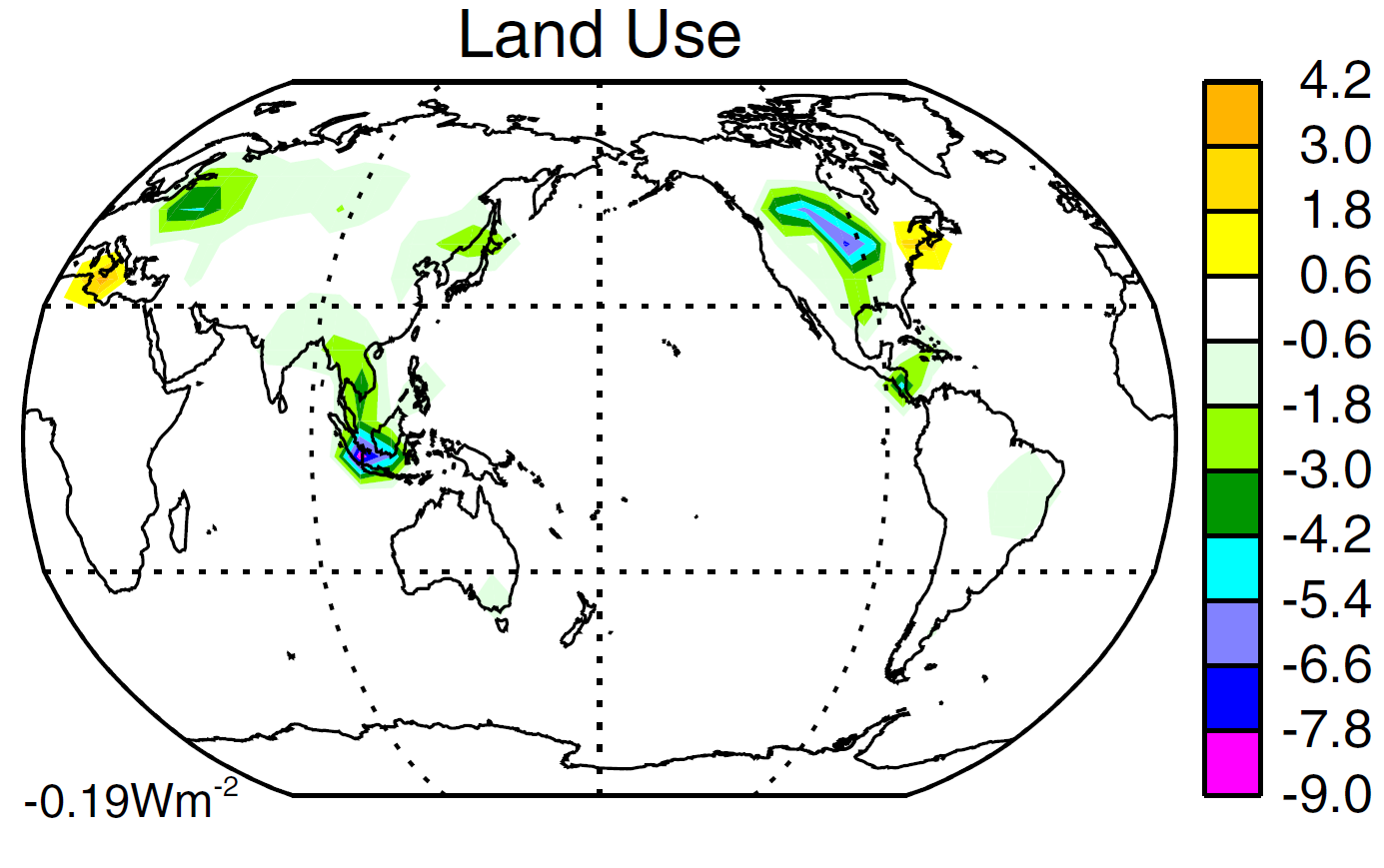
Figure 1. Reproduction of Figure 4c from Miller et al 2014: LU forcing in 2000 (vs 1850)
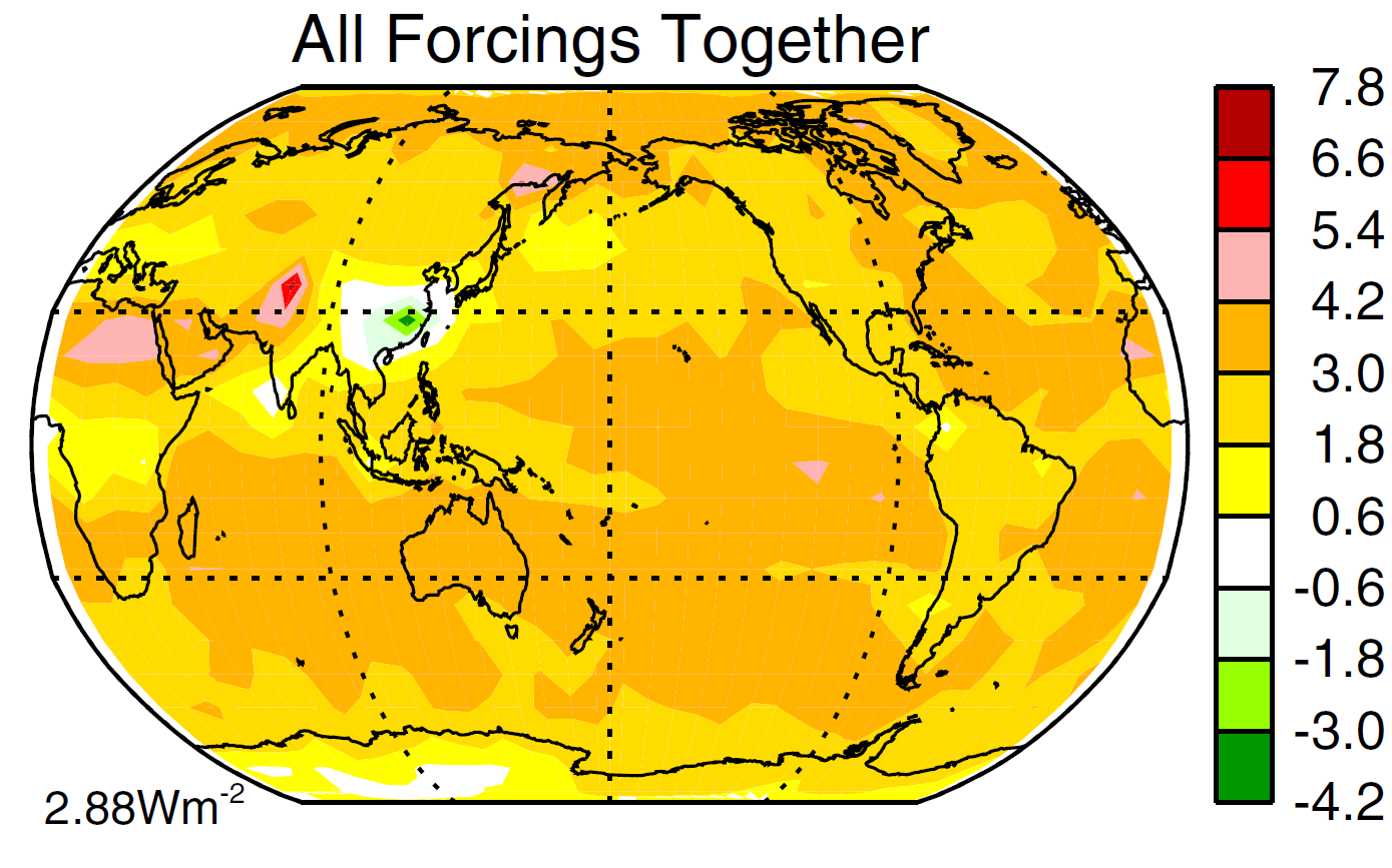
Figure 2. Reproduction of Figure 4d from Miller et al 2014: Historical forcing in 2000 (vs 1850)
b) There must be an error in the model radiative transfer code
The link given for this is to a comment of mine at Climate Audit, where I said:
““The GISS-E2-R increase in GHG ERF is 3.39 W/m2. The 1850-2000 increase in GHG RF and ERF per AR5 Table AII.1.2 is 2.25 W/m2, but I use the higher 1842–2000 increase of 2.30 W/m2 since the 1850 CO2 concentration in GISS ModelE2 was first reached in ~1842”. If one strips out the CO2 contributions, of 1.38 W/m2 for AR5 (based on an F2xCO2 of 3.71 W/m2) and of ~1.53 W/m2 for GISS-E2-R (based on an ERF F2xCO2 of 4.1 W/m2) the contribution of the other long lived GHG is 0.92 W/m2 per AR5 and ~1.86 W/m2 for GISS-E2-R.
That is, methane, nitrous oxide, CFCs and minor GHGs add TWICE as much forcing in GISS-E2-R as per the AR5 best estimate.
As I wrote, it looks as if GISS-E2-R radiative transfer computation in GISS-E2 may be inaccurate.”
When I write “may be inaccurate”, I mean just that. I do not mean, as Gavin Schmidt implies I do, that “there must be an error”. Moreover, far from making a claim based on no evidence, I set out in detail the evidence that it was based on.
The divergence is slightly smaller using the corrected ERF F2xCO2 value of 4.35 W/m2: ERF attributable to about non-CO2 greenhouse gases is then about 190% higher in GISS-E2-R than it is according to AR5. Gavin Schmidt has not attempted to justify the large difference, or to refute my calculation.
c) My alleged suggestion that it is statistically permissible to eliminate outliers in the ensembles because I didn’t like the result
This is quite wrong. I made no such suggestion, and Schmidt cites no evidence that I did so. What I wrote about the extreme outlier LU run 1 in my original article was this:
“It appears that the very high (although not statistically significant) best estimates for LU efficacy are affected by an outlier, possibly rogue, simulation run…. The difference from the ensemble mean is over four times as large as for any of the other 35 simulation runs. The LU efficacies estimates are greatly reduced if run 1 is excluded.”
In my second article I expanded on the issue as follows:
“Whatever the exact cause of the massive oceanic cold anomaly developing in the GISS model during run 1, I find it very difficult to see that is has anything to do with land use change forcing. And whether or not internal variability in the real climate system might be able to cause similar effects, it seems clear that no massive ocean temperature anomaly did in fact develop during the historical period. Therefore, any theoretical possibility of changes like those in LU run 1 occurring in the real world seems irrelevant when estimating the effects of land use change on deriving TCR and ECS values from recorded warming over the historical period.”
Maybe Gavin Schmidt doesn’t understand this point. My case for considering excluding LU run 1 has nothing to do with whether I like the result of the run or not.
Schmidt’s reworking of the Otto et al. results
A final point. Gavin Schmidt writes:
“If one was to redo those papers, you would choose the efficacies most relevant to their calculations (i.e. the ERF derived values for Otto et al) along with their adjustment for the ocean heat uptake (in our sensitivity test), and conclude that instead of an ECS of 2.0ºC [likely range 1.4-3.2], you’d get 3.0ºC [likely range 1.8-6.2].”
This is wrong. It appears he doesn’t understand that the underlying forcing estimates used in Otto et al. are not simple ERF values. Rather, they were calculated from the GMST response of CMIP5 models, their effective climate sensitivity parameters and their radiative imbalances. Since they reflect the actual model responses to the applied forcings, they already incorporate efficacies. If volcanic forcing produces only half the GMST and radiative imbalance response in CMIP5 models as does the same forcing by CO2, for instance – implying that volcanic forcing has an efficacy of 0.5 for the measure of forcing used – then the calculation of total forcing involved will automatically down weight by 50% the contribution from volcanic forcing.
[i] Hansen J et al (2005) Efficacy of climate forcings. J Geophys Res, 110: D18104, doi:101029/2005JD005776
[ii] Paraphrased from IPCC AR5 Annex III
[iii] Miller, R. L. et al. CMIP5 historical simulations (1850_2012) with GISS ModelE2. J. Adv. Model. Earth Syst. 6, 441_477 (2014). Open access.
[iv] Shindell, DT (2014) Inhomogeneous forcing and transient climate sensitivity. Nature Clim Chg: DOI: 10.1038/NCLIMATE2136
[v] It is also 86% for well-mixed greenhouse gases (GHG), and similar at 85% for aerosols. But it is only 80% for land use, 82–83% for solar and volcanoes, and it is 90% for ozone forcing.
[vi] The exception being for land use forcing, where the heat uptake has the opposite sign to the GMST change.
[vii] Transient efficacy for Historical (All forcings) would decline, from 0.96 to 0.85, but this may be affected by the issue of whether LU forcing was included in the measure of Historical forcing.
[viii] https://climateaudit.org/2016/01/21/marvel-et-al-implications-of-forcing-efficacies-for-climate-sensitivity-estimates-an-update/
[ix] niclewis I’m unsure why this reference given at RealClimate was to my web pages.
[x] See https://climateaudit.org/2016/01/21/marvel-et-al-implications-of-forcing-efficacies-for-climate-sensitivity-estimates-an-update/#comment-766295


78 Comments
“…If one was to redo those papers, you would choose…”
That’s like fingernails on a chalkboard. I had to visit RC to confirm it was quoted verbatim…which was worse than fingernails on a chalkboard.
I wonder if a correction will take place on behalf of the International Man of Mystery?
It appears, as usual, that Gavin Schmidt’s definitions are whatever he wants them to be at any given moment.
I asked him some honest questions myself once, and all he did was misdirect and toss about straw men. He simply wouldn’t give me a straight answer about anything.
See RC post “The tragedy of climate commons”. I ask that it looks like he has distributed emissions incorrectly, and he responded that the fishermen referred to population, not countries. So then I pointed out that his numbers still made no sense, and then he started trying to recover by distributing countries’ populations around.
Nic, you say:
Unfortunately, this is standard operating procedure at realclimate. In my experience with them, their usual practice has been to not quote directly, instead using inaccurate paraphrase to create a caricature of the original point.
As soon as I read that Gavin had paraphrased Nic’s points, and realised that he had provided no quotes, I had exactly the same thought.
Not just at Climate Audit. I’ve had many hundreds of conversations with activists (including activist scientists) about climate issues — most use this tactic, repeatedly and casually. They incorrectly represent what I’ve said and give a rebuttal to their strawmen.
When overused it gives the impression of talking with someone who is debating with the voices in his head. Or trying to talk with a guy in the park who is ranting from atop an orange crate.
I have also experienced this behavior, not just occasionally but regularly, on the part of climate alarmists.
It’s almost like they’re all reading from the same playbook.
Oh, wait… they are:
https://en.wikipedia.org/wiki/Rules_for_Radicals#Themes
Especially numbers 5, 8, 9 11, 13. They keep trying to push #3 but to their dismay they have learned that there are a lot of “experts” who are not following their dogma.
Agreed. SOP with all AGW advocates, in my experience. They must misrepresent your position, otherwise they cannot rebut.
This is my experience too. A lot of time is spent by activists arguing about implications and subtleties of language and exactly what was said and much less time on substance. My comment on “modelers are very clever and know the effect of modeling choices on emergent properties” aroused an emotional reaction but no substantive response a few posts ago here from Ken Rice
He totally ducked the question on whether land use run 1 was related to the ocean circulation error in GISS. Or whether such error still exists.
If one wanted to find the average height of humans and your 5 samples included Manute Bol it would be ridiculous to assert that made no difference to the results.
Wouldn’t the chance inclusion of Manute Bol in your small sampling size cause an honest investigator to reconsider the results?
Another example why “peer review” is a thing of the past since Al Gore invented the intarnet…
‘That the regression slopes involved will change, radically for LU, is obvious from the graph in Gavin Schmidt’s Ringberg15 presentation. It is less obvious from the equivalent graph in MEA15, as there the area around the origin is obscured by large decadal-mean blobs.’
Perhaps you could edit the post to show the ‘before and after’ comparison?
Before, slide 9 of the presentation:
Click to access Schmidt_25032015.pdf
After, the charts in MEA15. The blobs are so big it’s hard to tell if the lines cross the origin or not.
Steve: Inserted for comparison in this comment.
Is it at all possible that those big blobs are in fact meant to be meatballs to go along with the spaghetti?
Climateballs, perhaps?
May the Schmidt be with you!
It could be, but who in their right mind woud add meatballs before the spaghetti has even been cooked?
Regarding the fact that the regression lines don’t cross the origin, Gavin said in the comments section of the previous article:
‘You should note that there are lags in the system that extend beyond a decade. Thus expecting each decade’s temperature and forcing to line up perfectly is too optimistic. Instead, one expects temperatures to lag forcing by some amount and this leads to a small shift in the temperatures w.r.t. the forcing. An alternate way of doing the calculation (using the last decade minus first decade) is effectively equivalent to forcing the regression through the origin and was tested in the paper – it does not significantly impact the results.’
At first thought this doesn’t make much sense to me. The regression line that most obviously doesn’t end in zero is land use forcing. But why would the first two land use decadal blobs, which represent negative forcing, result in positive temperature change, even if small? You would expect a small negative forcing to result in a small negative temperature change, not the opposite. (My understanding is that the first blob in the charts above represents 1906-1915, not 1850-1859 – that’s why there are 10 circles for each forcing).
I readily confess my incompetence when interpreting this stuff, so I gotta ask, is what Gavin says true?
Reblogged this on The Ratliff Notepad.
This demonstrates Schmidt’s limitations when faced with questions from competent scientists.
Nic,
Very nice post; as usual, clear and straightforward.
The missing contribution of LU forcing in central North America in the all-forcings graphic (Miller 2014) is painfully obvious. I am sure there is some kind of error involved. Otherwise, one has to invoke herds of unicorns resident in central North America which generate a magical positive forcing exactly offsetting the negative local LU forcing.
Gavin’s refusal to admit the extreme LU efficacy comes down to accepting one very dubious run, a run which is a clear statistical outlier, goes to the heart of the problem with Marvel et al: the authors got results they ‘liked’ (lower efficacy for many forcings implies higher climate sensitivity… casting doubt on lower empirical estimates), and so failed to critically examine if their results might have errors. This is typical of the confirmation bias many highly motivated researchers suffer, and so not at all surprising. What is surprising (and more than a little disturbing) is that obvious problems/errors with Marvel et al were not addressed during peer review; this seems to me a recurring pattern in climate science. As some have noted, pal review is a poor substitute for peer review.
Finally, you wrote: “allowing for non-ocean energy absorption would increase most of the equilibrium efficacy and ECS estimates, typically by 5–10%.”
If the estimates of efficacies increased, does that not automatically mean the ECS estimate must decrease? Or am I missing something?
steve,
Their equilibrium efficacy for a forcing agent is defined as the ratio of (a) the ECS estimated, from the GMST deltaT response to the forcing change deltaF produced by that agent, using the energy budget equation [ECS = F2xCO2 x deltaT/(deltaF – deltaQ)]; to (b) the model ECS when forced by CO2, being 2.3 C.
So the ECS estimate and the efficacy estimate for a forcing agent are proportional. Their argument is that the mix of types of forcing during the historical period underestimate ECS in their model, corresponding to a composite efficacy of less than one. If that were the case in the real climate system, then estimates of ECS from observed changes in GMST and total forcing during the historical period would underestimate true ECS, which relates to pure CO2 forcing. In future, changes in CO2 forcing are expected to dominate totla forcing to a much greater extent than up to now.
The effect of allowing for non-ocean energy absorption is to increase the deltaQ term, reducing the denominator and hence increasing the ECS estimates. Along with the corrected value of F2xCO2 being higher than the one used in the paper, and the correct comparison being with the model’s effective climate sensitivity of ~2.0 C, this results in a higher estimate of equilibrium efficacy from Historical total forcing. As a result, the study would provide little evidence that historical period observational estimates of ECS have been biased low in relation to effective climate sensitivity.
Whether effective climate sensitivity is lower than ECS in the real world is a different question, which this study sheds no light on.
I read over Gavin’s post; once my eyes stopped rolling, two things stood out:
1) Gavin either can’t understand what Nic actually wrote, or he is willfully substituting straw men for most of Nic’s critiques.
2) Gavin’s parting comment about ‘other lines of evidence’ being consistent with Marvel et al is hollow. There are only two ‘lines of evidence’ which support high climate sensitivity… GCM’s, a dog’s breakfast at best, and ‘climate of the past’ based estimates, which can be most charitably described as what a dog’s breakfast is ultimately converted to.
The most solid evidence for the actual climate sensitivity is found in the best empirical estimates.
While I am not competent to understand the actual discussion, I will say this: it is very encouraging that Schmidt answered pretty much all of Lewis’ points, and with some detail. While some silly people (no offense, ATTP!) claimed, Why should scientists who published an important paper in a peer-reviewed journal be required to pay any attention to a blog post? – Schmidt and company seem to know better.
This is the way science is supposed to work, instead of Lewis publishing a rebuttal in about a year in a different journal, and Marvel et al publishing something else a year after that. Welcome to the new millenium: Schmidt has responded within weeks, Lewis has responded again within weeks, and probably when it settles down competent people will know who’s right on the various points within a few months. That’s as it should be.
Except he didn’t. He reshaped specific critiques into strawmen, and on 5 out of six points has failed to address the clear specifics Nic Lewis set forth. He probably cannot be ause then the paper crumbles completely.
Given that there’s much gnashing and wailing about Gavin not quite representing Nic’s point properly, I’ll point out that this isn’t a fair representation of my point. What I was getting at was that there can’t be an expectation of a response. Whether someone chooses to respond, or not, is up to them. It’s their choice. Given how this exchange is going, I’m not sure I quite see the point. It’s not looking like it’s going to converge in any meaningful way.
As far as this post goes, it’s not clear to me that this comment by Nic is correct.
The efficacy issue is relatively straightforward. Is the response to a change in forcing x, the same if the forcing is homogeneous, to when it is not homogeneous? What Nic is suggesting (I think) is that if you assess the forcing by considering the temperture response and radiative imbalances in a model, then that returns a result that incorporates the efficacy. I can see what Nic is suggesting, but I’m not convinced that this is necessarily correct. If Nic is correct, then I think that suggests that the regression used to estimate the forcings, does not quite produce a correct estimate of the forcing if the forcing is not homegeneous. However, it seems to me that if you were to introduce some kind of instantaneous change in forcing that was not homogeneous, then the basic analysis would still return a reasonable estimate for that change in forcing. I may be wrong, so I’ll have to think about this a little more.
“What I was getting at was that there can’t be an expectation of a response.” Which I addressed by using the word “required” in my paraphrase. Regardless, it’s beside the point. They are of course not “required”, whoever one can imagine doing the “requiring”. But as Gavin Schmidt and I and most of us understand, if they don’t respond people will think their work is wrong, and should.
“Given how this exchange is going, I’m not sure I quite see the point. It’s not looking like it’s going to converge in any meaningful way.” Huh? Marvel et al has corrected one point. The other five/whatever are currently in question. If these kinds of questions cannot be settled by competent statisticians, we’re all in a lot of trouble. I would submit that in that case a vast stretch of modelling is nonsense and none of us can trust a thing they produce, as we can’t even determine if their methods make any sense.
But why would you say that? It is now Schmidt etc.’s turn to respond. Either they will or they won’t. Is this just another way for you to say again, I support the AGW people’s claim that their work is correct without having to bother answering pesky objections by skeptics.
I expect that you’ll point out that you didn’t say that. But the rest of us indeed have an “expectation of a response”.
I had no expectation or hope of any response from Ken, but he chimed in nonetheless.
Apart from me not saying what you claimed I said, good point.
if they don’t respond people will think their work is wrong, and should.
IMO, thinking this, is particularly silly.
Yes, because I’ve indeed never said any such thing. It would be a particularly stupid thing to say.
Yes, I know, hence my point.
ATTP, I see you claiming constantly that you are being misunderstood. Whatever difference you see between your words and our paraphrasing of them, the rest of us apparently don’t see it. I guess we’ll have to continue to disagree on which of us is wrong about that.
” ‘if they don’t respond people will think their work is wrong, and should.’
IMO, thinking this, is particularly silly.”
Another thing we’ll have to agree to disagree about. If people don’t defend their work the rest of us are likely to think that they can’t.
Of course, this is aside from those who accept it because it supports their team.
Nic, it wasn’t clear to me from the post: how does Marvel et al’s correction to the forcings ultimately affect their estimates of TCR or ECS for CO2?
Their estimate of TCR based on Historical period iRF forcings increases from 1.2 C to 1.34 C, only marginally lower than the 1.4 C TCR of the model. Using ERF to measure forcing, the TCR estimate increases from 1.1 C to 1.29 C on my calculations (although they claim only 1.2 C). So there is no evidence that TCR is materialy underestimated when using historical observations.
For ECS, the Historical period iRF forcing based estimate increases from 1.63 C to 1.79 C based on ocean heat uptake alone, or to ~1.9 C based (correctly) on the total radiative imbalance. Although below the model ECS of 2.3 C, that is very close to the GISS-E2-R effective climate sensitivity of ~2 C, which is what this method would estimate if the forcing were purely from CO2.
Using the ERF measure, the ECS estimate increases from 1.72 C to 1.83 C on my calculations (from a clearly wrong 1.5 C to 1.8 C per MEA15/GISS’s corrections), or to 1.97 C based on the total radiative imbalance. So there is no evidence that effective climate sensitivity is materially underestimated when using historical observations. Although the model’s ECS is underestimated, that is only because its effective climate sensitivity increases over time. It has nothing to do with forcing efficacies.
I guess you can take this as Gavin’s answer to Nick’s very detailed points:
“My interest in going line by line is very limited”
So, Nicks analysis has caused Marvel to “correct” their paper on one count already, but the other six counts, well, he doesn’t have that much interest in going line by line. Is their another way to address the issues besides going “line by line”.
A very disingenuous man to say the least.
As on earlier occasions, Gavin Schmidt (aka the International Man of Mystery) did not include any acknowledgement in his correction.
Plagiarism is defined as “the “wrongful appropriation” of another author’s “language, thoughts,ideas, or expressions” and the representation of them as one’s own original work”.
Perhaps Nic should register a complaint with Kate Marvel, the lead author.
SM, that is a fair and good point, which you have appropriately made many times before. Perhaps its too painful for warmunists to acknowledge that knowledgeable skeptics such as yourself and Nic are watching, and in the internet era they cannot hide behind pal review. So they just quietly fix their grossest problems and pretend all is well.
Apparently in climate science, you only have to acknowledge your friends and political allies. Your political opponents? Not a chance. This apparently passes as normal in a pseudo-science, which once again shows just what is needed: defund all pseudo-science. That will solve the problem.
It seems that MEA15 needs an additional footnote acknowledging Nic Lewis’ posts on this blog.
Or perhaps this was another of those remarkable coincidences where the authors independently discovered their own error just moments before reading Nic’s comments?
“Discovered their own error just moments before reading Nic’s comments?”
Not “moments” before, as according to Nic:
“around the turn of the year I emailed GISS asking for the iRF and ERF F2xCO2 values. GISS have now finally revealed them, as 4.5 W/m2 for iRF and 4.35 W/m2 for ERF”,
So Gavin had a good heads up.
Gavin on Realclimate:
“I leave it to readers to judge who should be withdrawing their posts”
Yes, Gavin, rest assured, this is EXACTLY what readers are going to do…
Great comment. And true. Gavin reminds me of bubble boy syndrome.
It’s surprising serious people still consider Schmidt a reputable scientist. “By his deeds you shall know him.”
In his latest post at WUWT
Tim Ball mentions that GS was involved in the sue-them activities of the Greens: “I say this because I wrote the Foreword to the book Green Gospel and the author received a lawsuit filed on behalf of Gavin Schmidt in Washington State. The author informed me that the legal advice was just tell them to go away.”
You asked whether Gavin’s three-part statement “An alternate way of doing the calculation (using the last decade minus first decade) is effectively equivalent to forcing the regression through the origin and was tested in the paper – it does not significantly impact the results.” is true. Taking each part in turn:
1. “Using the last decade minus first decade) is effectively equivalent to forcing the regression through the origin.”
This is not generally true when, as in MEA15, the first decade used is 1906-15. And I can see no good reason for MEA15 using 1906-15 as the first decade for its regressions.
Nor is it true using the change from the origin, but in most cases this gives a result closer to that from regressing through the origin.
2. “was tested in the paper”
I can find no evidence in the paper that the effect of using the last decade minus first decade values was tested.
3. “it does not significantly impact the results”
Not so. To take the clearest case, transient iRF efficacy for LU forcing is 4.27 per the MEA15 regression. With the regression forced through the origin, the efficacy reduces to 1.18. Using the change from the origin to 1996-2005 gives an efficacy of 1.87, but using the change from 1906-15 to 1996-2005 gives an efficacy of 3.98.
That was Nic replying to Alberto Zaragoza Comendador.
Thanks, Richard. My machine crashed whilst writing the comment and, although WordPress saved the text, I didn’t notice that it had defaulted to the end position when I logged in again.
The validity of Schmidt’s assertion: “An alternate way of doing the calculation (using the last decade minus first decade) is effectively equivalent to forcing the regression through the origin and was tested in the paper – it does not significantly impact the results” seems like an important issue.
On the narrow issues of the “effective equivalence” of the two methods and whether the alternate was “tested in the paper”: in general terms, the two methods are clearly not “effectively equivalent”, though this doesn’t exclude the possibility that, by coincidence, they yielded similar results in a particular case, but this would have to be demonstrated. Like Nic, I see no evidence that this “effective equivalence” was tested in the paper and Schmidt’s claim to this effect appears to be flatly untrue. It seems implausible that they would have carried out such a test in the paper, since, if they had thought to do calculations with regressions forced through the origin, it’s hard to understand why they would then have used a kludgy and unsatisfactory method in preference.
It would be worthwhile asking Schmidt to point to the testing in the paper or alternatively provide details on how they carried out the test.
I suspect by ‘tested in the paper’, Gavin means ‘something similar was tested while we were working on the paper.’
something similar was tested while we were working on the paper
=============
and it didn’t give the result we wanted, so we “method shopped” until we found the answer we wanted.
so long as the author is free to chose any method they want to analyze the data, while rejecting any other method, the results will suffer from expectation bias.
for example: you are looking for gold. you try 4 different assay techniques and they are all negative for gold. You try a 5th technique and it shows positive for gold. You are going to stop right there and claim you have discovered gold.
what you have ignored is that if you tried 99 different assay techniques, only method 5 would show positive for gold. the other 98 would be negative.
what you should have concluded is that there is no gold, that method 5 was a false positive. however, in climate science this problem is ignored, allowing false positives to routinely be used as evidence of true positives.
you say:
actually that’s completely untrue. Mining promoters are required to disclose negative results. And, if you got negative assays using conventional methods, it would be illegal to not report them.
Going back to my initial entry into this field, I was very surprised both by Mann’s withholding of adverse verification r2 results and even more surprised by climate scientists not viewing this as a very serious misrepresentation (by omission). It’s an issue that Steyn (and Tim Ball) should pound mercilessly in their respective lawsuits. Even if a hockey stick like squiggle were subsequently established using different data and methods (and I’m doubtful of any supposed vindication from upside down sediments and cherry picked tree ring chronologies), that doesn’t vindicate the deception arising from the failure to disclose adverse statistics pertaining to the MBH reconstruction. The distinction is not evident to many “skeptics” who fantasize that a court can litigate the medieval warm period. A court cannot be reasonably expected to resolve such issues, but judges do understand the failure to disclose relevant adverse statistics – even if academics don’t.
One should establish an analytical protocol before conducting analysis…
eh…whats the use?
I have to say that the withholding of the adverse R2 results immediately struck me as a stand-out. However it did take the release of the original code to definitively establish that R2 had been calculated throughout. Even more egregious is that in the 1998-9 papers, Mann quotes R2 where it supports his conclusions (for example for the 1815 step) but omits it where it does not support them. That is, I believe, often regarded as an example of academic fr**d, which is distinct from common fr**d.
Didn’t Mann also rather cleverly avoid saying in one of the hearings whether he had calculated R2 by saying merely that it would be foolish to do so (or words to that effect) ? Pity that the chance was missed to get him to answer a straight question about it.
Steve: It was at the NAS workshop. In my opinion, Mann did not “cleverly avoid” answering; rather, he lied. Christy directly asked Mann whether he calculated the verification r2 statistic. Mann’s answer (See https://climateaudit.org/2006/03/16/mann-at-the-nas-panel/) was “We didn’t calculate it. That would be silly and incorrect reasoning”. The NAS panel had more than information to know that this answer was a lie. It had been one of the issues in our presentation the previous day. However, rather than cross-examining him on the lie, but the NAS panel sat there like bumps on a log.
At the workshop, for all other participants, there was an opportunity for non-panelists to ask questions. However, not for Mann, because Mann fled the workshop before any non-panelist (e.g. me) could ask him a question. When I subsequently had an opportunity to comment (after Mann’s precipitous exit), I criticized the panel for not following up, but to no avail.
Steve Mc: “judges do understand the failure to disclose relevant adverse statistics – even if academics don’t.”
I am not so sanguine about judges’ abilities in this area. If they could understand the statistical issues, they would generally require full disclosure. However, the statistical issues involved here are far beyond the understanding of most judges, who are, by virtue of the greatly varied nature of the cases they handle, generalists. If judges don’t understand the underlying statistical concepts, they can easily be fooled by deceptive arguments coming from people employed by what appear to be prestigious universities or organizations.
JD
Steve: let me try to make my point a different way as I have argued over and over against excessive expectations by “skeptics” of the legal system and do not wish to be perceived as having such expectations myself. I’m really trying to point to the issues that I think have the best chance of being understood by a judge who is giving deference to academics from prominent universities. Many “skeptics” seem to want to litigate the medieval warm period in the Steyn and/or Ball cases. In my opinion, this is a ludicrous expectation as any judge would be obliged to defer to the opinion of academics from prominent universities. In my opinion, there is a far, far better chance of getting a judge to take heed of the withholding of adverse verification statistics than to trying to decide a scientific issue because the withholding of material adverse information is something that arises in non-scientific contexts.
In saying “judges do understand the failure to disclose relevant adverse statistics – even if academics don’t”, I wrote quickly and did not express myself as clearly as I might have. I think that judges can be expected to understand the concept of failing to disclose material adverse information, since that’s a battleground issue in many securities cases and fairly conventional law. On the other hand, I’ve pretty much despaired of academics understanding this concept. You may recall the discussion with Pielke Jr where he attempted to distinguish “fudge” from “fraud” and pointed out that “fudging” was common practice in academia. I’ve consistently urged bloodthirsty “skeptics” to remember this.
My recommendation to lawyers in these cases would be to try to get the judge to focus on the withholding of adverse statistics as falling within the more general concept of withholding of material adverse information, trying as much as possible to keep the discussion as general as possible. I would point out that many familiar concepts such as “profit”, “return on investment” etc are also “statistics” and the withholding of adverse data of this type is treated harshly.
As you observe, a judge in such a case could “easily be fooled by deceptive arguments coming from people employed by what appear to be prestigious universities or organizations”. Presumably Mann’s side would argue that the withheld verification statistics were not “material”. But the job of the lawyer in these cases to focus as much as possible on issues where there’s a chance of winning. I still think that this is the strongest line of attack and much, much stronger than trying argue about the medieval period. That’s the point that I’m arguing here.
Also, in respect to the defamation cases – as you well understand – the point that needs to be established is a little different than in a misconduct case. It is a matter of fact that Mann withheld the adverse verification r2 statistics. In my opinion, it is entirely reasonable for someone to believe that this was a “material” omission, thereby getting to a “fair comment” defence. As I wrote previously, I think that Steyn’s case resolves more easily on the other issues that I’ve written about previously.
Steve,
I agree that withholding evidence is easier to demonstrate to courts than litigating the medieval warm period. However, I have a serious concern that the vast majority of courts would not understand the basics of statistics or the verification r2 statistic. If a court doesn’t really understand what r2 is, it will be very reluctant to find that the withholding of r2 is a serious issue.
Because I believe that courts have a difficult time understanding statistics, I have argued repeatedly that, in legal actions, people have to focus on 2 or 3 simple incidents of misconduct (such as Tiljander upside down, Mann lying about the excel file) if people wish to put a serious dent in the AGWers deceit and misconduct.
In confirmation of your observations, I would add that it is humorous to me that AGW “scientists” think they can withhold adverse information or data. All lawyers instinctively understand that even if the facts presented by someone are literally true, if only one side is presented such a presentation can be entirely wrong or misleading. This idea was expressed by New York’s chief justice in the 1980s when speaking about the one-sided nature of grand juries, he stated that he could indict a ham sandwich if he wished.
JD
Steve: in a litigation, I entirely understand and agree with your point that “people have to focus on 2 or 3 simple incidents of misconduct”. A wise old litigation lawyer explained that to me many years ago. Reasonable people can disagree about the right 2-3 incidents. You’re familiar with both the incidents and the law and your views on this ones that I would take very seriously if it were me in the litigation. Interesting that you bring up the excel incident. I was dumbfounded by Mann’s original lie about the excel file and it definitely changed my perspective on Mann. It’s somewhat tangential to the science issues and has little academic traction, but is an easily provable lie.
I had 2-3 incidents in mind when I mention the verification r2 statistic. Notwithstanding your concern about its relevance getting fogged by academics, it would still be in the 2-3 incidents that I’d recommend to the libel litigants. The issue was fundamental to my own viewpoint about the ethics of MBH98 and my perspective is relevant. Also, Mann was asked about it by the Energy and Commerce Committee and subsequently by the NAS panel – to whom he once again lied about it.
It also depends on purpose. I was commenting here in the context of the Steyn and Ball libel actions, rather than trying to prove “AGWer deceit and misconduct”. I think that Steyn and Ball’s libel defences are better off focusing on whether Mann had been deceptive in his hockey stick, rather than trying to litigate wider issues – a point on which I’m sure that we are in agreement.
In my own writing, I’ve been careful not to avoid thinking in terms like “AGWer deceit and misconduct”. I think that there are certainly such indidents – one need think no further than Peter Gleick – and, in my opinion, the acquiecence of AGWers in such conduct has done their cause no good, but I’ve always taken care not to over-generalize and to emphasize that there are many competent scientists who view the situation with concern. Again, I don’t think that there is any actual disagreement between us on this point.
Nic, my estimates of the uncertainties for the efficacies of the forcing agents relative to GHG for the Marvel derived iRF and ERF approaches indicated that the uncertainty levels were such that only Volcanic (lower) and AA (higher) agents could be said to be different than GHG. Given the GHG and AA CIs it would not take much of a change in AA to have no statistical difference there.
Would you care to comment and also talk about the uncertainties seen in the Marvel approach versus your approaches used in your publications?
Ken, I’m not sure the uncertainty in the iRF efficacy estimates is as high as you suggest, if one calculates them using the MEA15 basis. As I wrote in this post, the correct single forcing uncertainty ranges are only half those given in the corrected SI that Gavin has made available.
In my observationally-based studies, observational uncertainty is substantial. It plays no part in a model based study like MEA15, as the model simulation outputs are known exactly, in all grid cells. It is only internal variability in the model that is involved. In my studies, I allow for internal variability in the real climate system, usually based on that in long unforced AOGCM control runs, as the observational record is quite short.
However, MEA15 does not seem to have made any allowance for uncertainty in F_2xCO2. That must exist, but perhaps is not very large.
Nick writes
Using this argument, the results only apply to the model and not the real world.
Yes, the MEA15 results, even if correct, would only apply to the GISS-E2-R model – indeed, to it as it was before the ocean mixing error was corrected.
The MEA15 results would only apply to the real world if the model behaved very similarly to the real world in all relevant respects – which seems less than certain, to put it mildly. That is why I consider the conclusion of MEA15, that “Climate sensitivities estimated from recent observations will therefore be biased low…” to be unjustifiable, whether or not the study contains serious errors (as it does).
In my comment above I should have pointed to my surmise that the Marvel approach in looking for statistically significant differences in forcing efficacies is limited by the noise in the temperature series from the individual forcings. I am not sure if this same limation is as critical in other approaches.
Forcing uncertainties, particularly for aerosols, are the biggest issue for instrumental observation based TCR and ECS estimates. Efficacy uncertainties are thought (per AR5) to be a large exent allowed for when ERF estimates are used, except for black carbon on snow.
Heat uptake uncertainty is the next biggest component of uncertainty in instrumental observation based ECS estimates. Uncertainty in GMST, and in F_2xCO2, are lesser components.
Nic, I modeled the white and red noise of the GISS E2-R climate model from the temperature series produced by the individual forcings used in Marvel and from that model did simulations to determine confidence intervals (CIs) for the ratio of deltaT/delta F. I did the same for the ensemble averages. The obvious alternative involves using the outputs of a reasonably large number of multiple runs from a climate model and estimating the CIs from the distribution of those runs.
Since we can never have more than the single observed realization of the earth’s climate, estimating the CIs of the observed outputs necessarily requires modeling the noise and using simulations. Without the use of a noise model to compare model and observed outputs, the alternative here is to use the output of a reasonably large number of multiple runs of a climate model and determine where the observed output fits with the model run distribution.
In order to obtain the most from this exchange in my view, Gavin Schmidt’s comments and replies to Nic should not be generalized to somebody’s view of how a person with a strong advocacy position on AGW would respond, but rather what do his responses say about the matter at hand and how well the points that Nic brings to the fore are really understood and covered in Marvel. The exchange is also valuable in getting all the misunderstandings about unclear comments in the paper from a reasonable and knowledgeable reader resolved and out of future discussions.
Gavin’s appearance of an ego and a tendency towards being dismissive may be getting in the way of some of his replies and needs to be considered in why he misinterprets some of Nic’s criticisms and queries. A protracted discussion would eventually resolve these matters, but that might not be on the agenda for Gavin.
Yes, but who is going to help Gavin to correctly grasp the specifics of the points raised by Nic, assuming that that the problem is indeed one of inability to “grasp”.
Nic, are there any strategies or approaches that might be used to keep your exchange with Gavin Schmidt on point so that you can be satisfied that Schmidt has truly addressed the issues you have posed? What about the coauthors?
Ken, Gavin Schmidt has not addressed most of the issues I raised, and I expect he has no desire to do so as that would (on my analysis) involve admitting further serious deficiencies in the paper, negating its main conclusions.
Gavin Schmidt is the boss at GISS; it is a government agency not a university with semi-independent academics. So I doubt that co-authors feel able to respond freely to me, although I have had some sensible and good-tempered correspondence with Ron Miller. I believe Kate Marvel is on leave.
I hope the irony here is not lost that Schmidt replaced Hansen when he retired recently and Nic has commented on two studies,one by Hansen and the other co-authored by Schmidt that show very different evidence for the ratios of forcing agent efficacies.
I wonder what Hansen’s thoughts are on Marvel vis a vis his paper on the same topic. I also wonder if GISS being a US government agency might feel obliged to reply in full to a US citizen and perhaps less so to a non citizen of the US. Their obligation would be more politically than scientifically motivated in that case.
Nic: Does all of these corrections to forcing make good scientific sense to you?
Back in the dark ages, there was a single answer for the forcing for 2XCO2: 3.7 W/m2. I believe the proper name for this quantity is now iRF. This quantity was calculated for today’s earth with the best estimates of temperature and composition profiles for various regions on the planet (soundings), cloud cover, cloud top elevation, etc. It was the instantaneous change in radiative imbalance at the tropopause, because stratospheric adjustments were expected to negate any change in OLR caused by increasing GHGs above the tropopause.
Herein you are discussing an iRF for 2XCO2 of 4.5 W/m2 for the GISS, about 20% higher. This is a non-trivial difference: 20% of a doubling is the forcing difference between 400 ppm and 460 ppm. Do all current AOGCMs predict that iRF is much higher than 3.7 W/m2? Are the planetary atmospheres through which these forcings are calculated that different from each other and from the assumptions behind 3.7 W/m2: Different absolute humidity in the upper troposphere? Different albedo? Different cloud top altitude.
Strictly speaking (COE), all W/m2 are created equal and are converted to temperature using the same heat capacity. Why should the efficacy of methane forcing differ from the efficacy of CO2? Overlap with water vapor is important for radiation from clear skies, but shouldn’t all models should get relative humidity correct and agree with observations from space? Methane does produce some stratospheric water vapor in AOGCMs and therefore a forcing slightly different from simple radiative transfer calculations.
Don’t anthropogenic aerosols directly impact only reflection of SWR through clear skies with similar fractional cloud cover in all models? Aren’t they removed by precipitation in regions with rising air therefore not important above most cloud tops? The amount of indirect aerosol effect can obviously vary from model to model, but reflected SWR still needs to agree with current satellite observations.
Doesn’t land use change only effect surface reflection through clear skies with similar fractional cloud cover in all models?
Is there something I can read that would make me more comfortable (and possibly less ignorant) that all of these corrections arise from physically sensible phenomena and are absolutely essential obtaining the best estimate for ECS using historical forcing and temperature?
Frank, I would read Hansen et al 2005: Forcing efficacies; it can be found non-paywalled. It is a far more thorough study than MEA15, and despite using the similar, albeit earlier, GISS ModelE2 it came to very different conclusions than MEA15.
I think forcing from stratospheric water vapour, including that from oxidation of methane, is normally accounted for separately from methane forcing.
The 3.7 W/m2 in IPCC Ar4 and AR5 came originally from Myhre et al 1998 and is a stratospherically adjusted forcing or RF, not an iRF.
The GISS scientists have so far been unable to establish why global CO2 iRF in thier ModelE2 is ~15% higher than in ModelE, mainly arising outside the tropics. (See Miller et al 2014 p.449; this study has lots of good information about forcing during the historical period in GISS ModelE2.
Some troposheric aerosols absorb radiation, e.g black carbon. And the LW aerosol direct effect is not negligible (~+0.25 W/m2), although sometimes excluded. Satellite observations may be able to constrain present day indirect aerosol forcing, but there is considerable uncertainty in the preindustrial level of forcing.
I believe that land use change forcing in all or most models is primarily due to SW albedo change.
Correction: I meant to say “global WMGHG iRF in their ModelE2 is ~15% higher than in ModelE”, not that global CO2 iRF is ~15% higher.
I also meant to say that Hansen et al 2005 had used the earlier GISS ModelE; it is MEA15 that used GISS ModelE2 (in the E2-R NINT version).
Boisier, et al (2013) would seem to confirm your point:
Well, in his mind he has to save some face.
I have not studied this article, but I note that throwing mud around saves some face, in some people’s minds anyway.
Just for the record, I left this comment on RealClimate, although it has not appeared as yet.
Paul_K says:
Your comment is awaiting moderation.
20 Feb 2016 at 1:05 AM
Gavin,
There appear to be a couple of issues which have been raised to which you have not yet responded. I have a few more questions arising from your latest results but this comment is already weighty enough.
a) Thank you for the correction and release of the ERF and Fa values for CO2. So far, you have provided a single corrected Fi value for 2xCO2, but have not yet provided any information on the relationship between Fi and concentration. The recently released data for ERF and Fa suggest a curve shape which is markedly different from Hansen 2005. Whereas on a plot of forcing vs log of relative concentration, Hansen showed a relationship which was concave upwards, the limited ERF and Fa data you have supplied for GISS-E2-R suggest a relationship which is concave downwards. I would be very grateful if you were to release your Fi values vs relative concentration upto 4xCO2, or at the very least your point 4xCO2 value. As I explained in an earlier request on 12th January, these data are critical to test that the aggregate response of GISS-E2-R conforms reasonably to your explicit assumption of a linear system.
b) There are three lines of evidence which suggest that the LU forcing agent was not correctly switched on when you calculated the Fi values for the Historical simulation, none of them conclusive but each highly indicative. Can you please provide your assurance that this has been tested and that there is no doubt that LU forcing was included in the “All-forcings_together” values? [For the avoidance of any doubt, the question is not, repeat not, whether the LU forcing agent was switched on during the Historical simulation. I can and have independently verified this.]
c) Both you and Dr Miller remarked in published papers in 2014 that an error had been identified in ocean heat transport in GISS-E2-R. Can you confirm that the results in the public domain have been corrected for this problem? If so, can you provide a pointer to the correction? If not, can you explain why you are confident that this error should not influence the values which you have used in Marvel et al?
d) If your CI values purport to be based on variance of the mean, they appear to be out by a factor of about two. [This is not a problem arising from the difference between Guassian and t-distribution.]
e) You appear to have sidestepped the key issue raised by Lewis with respect to your introduction and definition of “Equilibrium Efficacy”, which is that it confuses two quite separable concepts. Normally when new measures are invented by scientists and engineers their utility arises from their ability to elucidate, not to confound. Your definition specifically confuses the question of the efficacy of a forcing agent with the question of why there is a difference displayed in GCMs between their effective equilibrium temperature and their reported equilibrium temperature. The latter difference arises from the fact that most GCMs display “time-varying feedback”, which results in a curve on a Gregory plot rather than a straight line. We now know from Andrews 2014 that a key culprit for this curvature in most models is SW CRE; hence we still do not know whether this is entirely an artifact of cloud parameterization or whether such curvature represents a real-world phenomenon. If you wish to present an argument that it IS a realworld phenomenon, and hence observation-based methodology underestimates ECS, then by all means do so, and we can have an intelligent debate. However, let us not confuse that conversation with the question of efficacy. If I take the GISS-E2-R 1% p.a. data – the basis for your transient efficacy denominator – then I find the gradient of an F-N vs T plot (still using Hansen’s Fi data to define the F vs time relationship) is 2.28 W/m2/deg K. The data from the historic run, on the other hand, yields a value of 2.39 – almost identical. Hence, we might reasonably conclude that there has been no significant change in estimated effective equilibrium temperature, a very different picture from the result you obtain with your definition. The CO2-only case yields an estimate of Teq for 2xCO2 of 4.52/2.28 = 1.98 deg K. This compares with the reported ECS of 2.3 deg K. Hence, using your definition we find that CO2 has an Equilibrium Efficacy of 1.98/2.3 = 86%. So we deduce that CO2 has an Equilibrium Efficacy of only 86% relative to itself. You must see that this is an absurd result.
Hi Paul, Just wanted to point out that Gavin responded to your post in case you haven’t seen it yet: http://www.realclimate.org/index.php/archives/2016/02/marvel-et-al-2015-part-iii-response-to-nic-lewis/#comment-643235
Steve,
Whatever happened to point 3 in your post?
JohnA,
It’s my post, not Steve’s.
Point 3 was dealt with in the second paragraph. It would have been clearer if I had stated that the point involved was number 3. But I did start the next paragraph with “I will now deal with Gavin’s responses to the remaining five of my six points, using the same numbering”.
Reblogged this on Canadian Climate Guy.
4 Trackbacks
[…] published online (as here), it has been kept available alongside the corrected version. – Click here to read the full article […]
[…] Nic Lewis schools Gavin on climate sensitivity at Climate Audit [link] […]
[…] A Return to Polar Urals: Wilson et al 2016 By Steve McIntyre, Climate Audit, Feb 8, 2016 https://climateaudit.org/2016/02/08/… “The Briffa 2013 MXD chronology, though lacking a distinctive HS [Hockey-Stick] shape, is nonetheless the produce [product] of an unintelligible and bizarrely complicated series of adjustments. Ironically, these adjustments produce a chronology that is functionally indistinguishable from a chronology of annual effects produced from a random effects model – further supporting the longstanding Climate Audit thesis that analysis of tree ring data ought to be done within the framework of random effects statistics.” Marvel et al. – Gavin Schmidt admits key error but disputes everything else A guest article by Nicholas Lewis, Climate Audit, Feb 11, 2016 https://climateaudit.org/2016/02/11/… […]
[…] I responded to the RealClimate article, here, I inter alia presented further evidence that LU forcing hadn’t been included in the computed […]