A guest article by Nicholas Lewis
Introduction
In a recent article I discussed the December 2015 Marvel et al.[1] paper, which contends that estimates of the transient climate response (TCR) and equilibrium climate sensitivity (ECS) derived from recent observations of changes in global mean surface temperature (GMST) are biased low. Marvel et al. reached this conclusion from analysing the response of the GISS-E2-R climate model in simulations over the historical period (1850–2005) when driven by six individual forcings, and also by all forcings together, the latter referred to as the ‘Historical’ simulation. The six individual forcings analysed were well-mixed greenhouse gases (GHG), anthropogenic aerosols, ozone, land use change, solar variations and volcanoes. Ensembles of five simulation runs were carried out for each constituent individual forcing, and of six runs for all forcings together. Marvel et al.’s estimates were based on averaging over the relevant simulation runs; taking ensemble averages reduces the impact of random variability.
In this article I will give a update on the status of two points I tentatively raised in my original article.
Land use change (LU) forcing
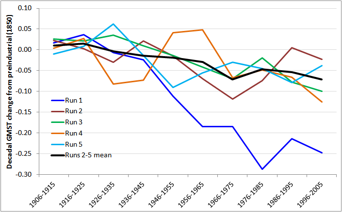
I commented in my original article that LU run 1 showed a much more negative GMST response than any of runs 2 to 5, from the middle of the 20th century on (see Figure 5 in the original article). I conjectured that run 1 might be a rogue. Excluding it reduces the transient efficacy for iRF from 3.89 to 2.48, and that for ERF from 2.61 to 1.75, with both iRF and ERF equilibrium efficacies reduced to around one.
I have now downloaded and processed CMIP5 data for the GISS-E2-R single forcing runs, so I can show the spatial effects of LU forcing on simulated surface temperatures.
First, I show (Figure 1) the spatial distribution of Land use forcing applied in the model simulations during 2000. Its global mean value is −0.19 W/m2, but the forcing is very concentrated in particular regions. The forcing increases gradually from zero in 1850, flattening out after ~1960.
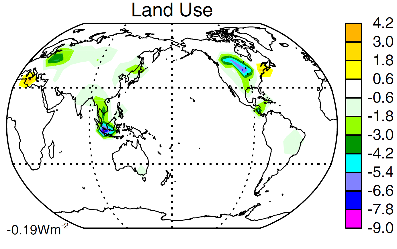 Figure 1. Reproduction of Figure 4c from Miller et al 2014:[2] LU forcing in 2000 (vs 1850)
Figure 2 shows the changes simulated by GISS-E2-R in response to LU forcing for each of simulation runs 2 to 5. They compare mean temperatures over 1976–2000 with those over 1850–75. Note that longitudes in these world maps are centred on Greenwich rather than the Pacific.
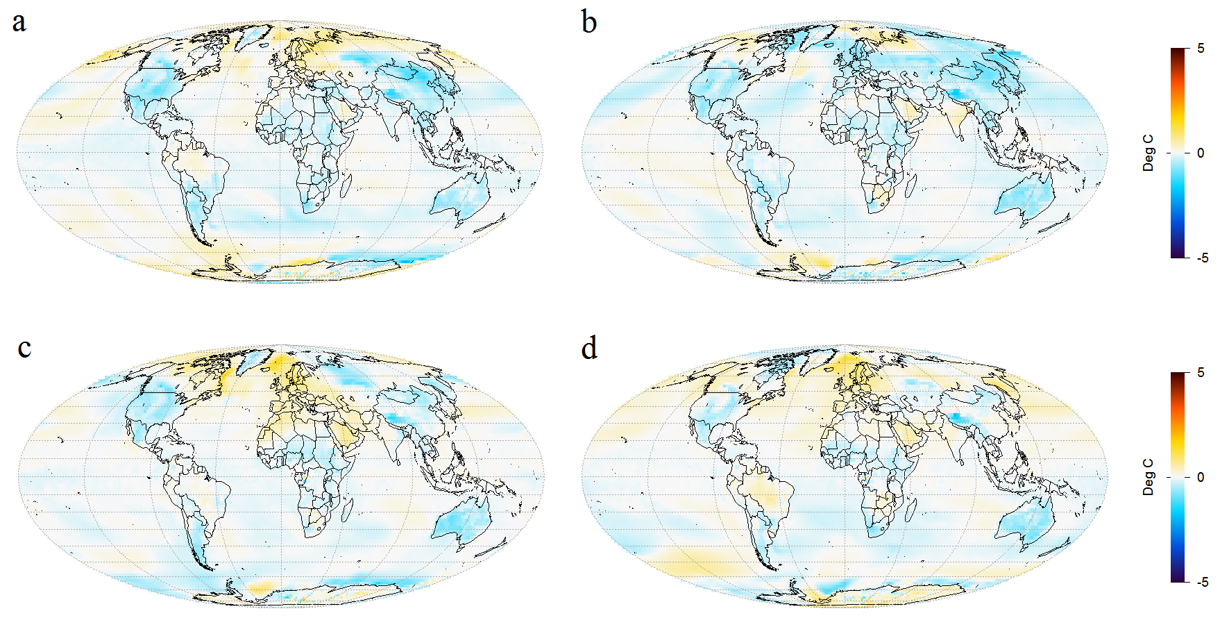
Figure 2. Simulated surface temperature change (1850–75 to 1976–2000 mean) driven by land use change forcing only: maps a to d show results from runs 2 to 5 respectively.
As the forcing and resulting temperature changes are small, internal variability has a significant effect on simulated changes even when comparing 25 year means, with changes varying in sign over some land areas and most of the ocean. Figure 3, which shows the average of all the plots in Figure 2, confirms that temperature changes are small everywhere. Globally averaged, there is a cooling of 0.04°C. Note that the temperature scale has been halved in Figure 3; taking the average of four runs halves variability.
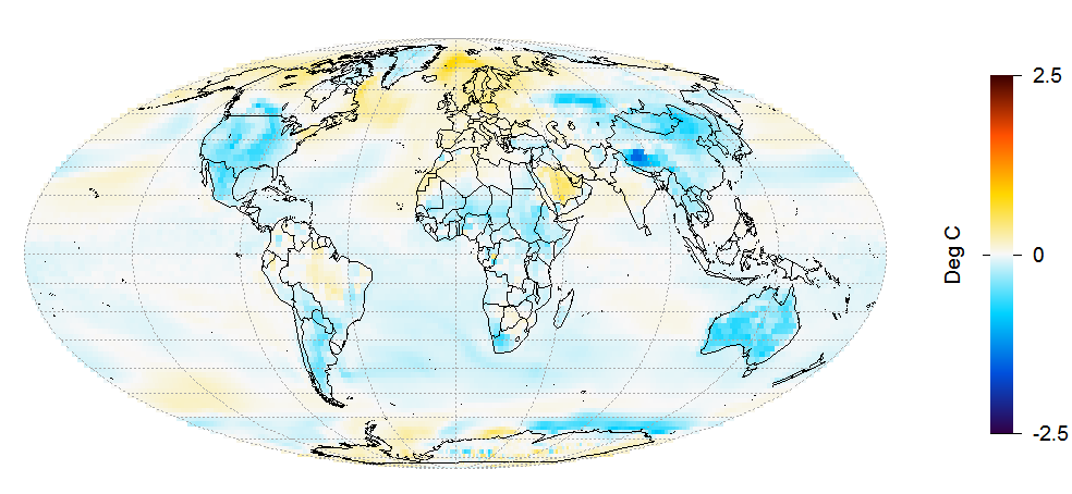 Figure 3. Average of temperature changes for runs 2 to 5, as plotted in Figure 2.
Figure 3 also shows that although LU forcing is very spatially inhomogeneous, it affects temperatures throughout the globe. The generally greater cooling in land masses than over the ocean is mainly due to temperatures over land generally being more sensitive to global forcing, not to LU forcing being located in land masses. Broadly, in GCMs a local forcing has a global effect, with local temperature changes being determined more by local climate sensitivity (the reciprocal of climate feedback strength) than by local forcing. Forcing from black carbon deposited on snow is a partial exception to this rule; it is concentrated at high latitudes, from which heat is less readily transported elsewhere. The way in which GCMs spread globally the effects of local forcings accords quite well with a physical understanding of how the climate system works. And it explains why, when a measure of forcing (ERF) that allows the troposphere to adjust to its presence is used, most forcings are thought to have an efficacy close to one despite some of them being quite spatially inhomogeneous.
The temperature changes simulated in run 1, shown in Figure 4, are very different.
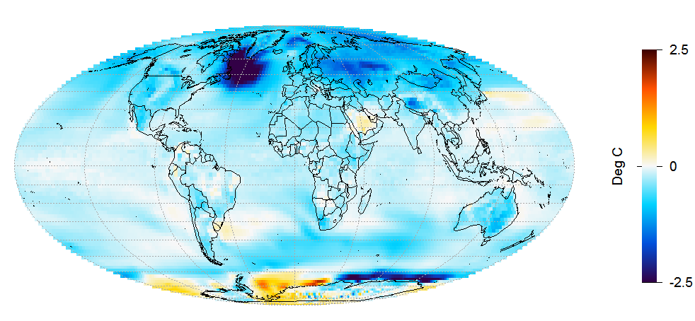
Figure 4. LU run 1 surface temperature change from 1850–75 to 1976–2000 mean.
A very cold anomaly has developed in the ocean south of Greenland. In most of the dark blue patch, the temperature has dropped by over 3°C, and by over 5°C in the centre of this area. Additional cooling to that shown in runs 2–5 has developed almost everywhere, apart from off Antarctica, where some areas have warmed strongly and others cooled strongly. This all seems to point to some major change in the ocean overturning circulation having occurred in this run, resulting in the cold ocean anomaly south of Greenland and substantial surface cooling in most areas.
I drew this finding to the attention of Ron Miller of GISS, one of the Marvel et al. authors, last week, asking whether he had any explanation and enquiring whether the simulation might be rerun, as GISS had done when another single forcing run had, for unknown reasons, an unreproducable excursion in the middle of the run. I have now heard back from Ron Miller to the effect that, although LU run 1 indicates greater cooling, he doesn’t regard the run as pathological and can’t see any reason to treat it differently, and that they don’t have any current plans to rerun this simulation.
Whatever the exact cause of the massive oceanic cold anomaly developing in the GISS model during run 1 , I find it very difficult to see that is has anything to do with land use change forcing. And whether or not internal variability in the real climate system might be able to cause similar effects, it seems clear that no massive ocean temperature anomaly did in fact develop during the historical period. Therefore, any theoretical possibility of changes like those in LU run 1 occurring in the real world seems irrelevant when estimating the effects of land use change on deriving TCR and ECS values from recorded warming over the historical period.
Possible omission of land use change forcing from Historical forcing data values
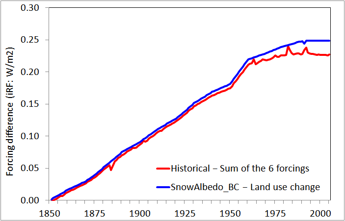
I noted in my original article that the differences between the GISS Historical forcing data (iRF time series) and the sum of those for the constituent individual forcings suggested that, unlikely as it might seem, the negative contribution from land use change forcing might have been omitted from the Historical forcing values. My Figure 4 showed that when LU forcing was deducted, the excess of Historical forcing over the sum of the six individual forcings analysed by Marvel et al. almost exactly matched forcing from black carbon deposited on snow and ice (Snow Albedo BC), a minor forcing included in the Historical simulations in addition to the six forcing analysed in Marvel et al.
Omission of LU forcing values would have increased Historical forcing values, thereby (assuming that LU forcing had nevertheless actually been applied in the Historical simulations) causing a downwards bias of ~5% or so in estimates of efficacy and TCR/ECS derived from the Historical simulations. By contrast, the inclusion in the Historical simulation forcing values of Snow Albedo BC forcing does not cause a bias since its effects on GMST and heat uptake are reflected in the Historical simulations; likewise for the trivially small (<0.0025 W/m2) orbital forcing. However, it is difficult to see how the Historical simulation could have included LU forcing without the value of LU forcing being included in the Historical forcing values. That is because, as I understand it from reading Miller et al. 2014, the Historical forcing values were derived from the Historical simulation radiation data, not by adding up individual forcing values derived from the constituent single forcing simulations.
Nevertheless, I decided to investigate this issue by multiple regression of Historical forcing against the constituent forcing series. This approach is based on the standard assumption that individual forcings are linearly additive. Although in reality any climate-state dependence of individual forcings would make this assumption inaccurate, here all the iRF values have been calculated with a fixed 1850 climate state, before perturbation by any applied forcings, so I would expect linear additivity to be a good approximation.
I used annual data over 1851–2012, being all data except for the baseline year of 1850, when all forcing values were zero. I started the regression in 1851 as there appeared to be a ~0.004 W/m2 jump in Historical forcing relative to the sum of individual forcings between 1850 and 1851. I therefore added 0.004 W/m2 to the Historical forcing values and then regressed with no intercept term. I started by regressing on all nine series: there are separate series for direct and indirect aerosol forcing. Table 1 shows the results.
 Table 1. Results from regressing all Historical forcing on all individual forcings over 1851-2012
Land use forcing has a regression coefficient negligibly different from zero, whereas all other forcings have regression coefficients close to one. This result provides further evidence that LU forcing may not be included in the Historical forcing values. The fit is extremely good: the residual standard deviation is under 0.1% of Historical forcing in 2000. However, given the similarity between most of the forcing time series – which apart from volcanoes and solar variation all increase smoothly over time – the estimation uncertainty will be greater than appears from the coefficient standard deviation values. Therefore, even though the modest excesses over one of the Aerosol-direct and Ozone coefficients are three or four times the standard deviation estimates, it is difficult to see them as being at all significant.
Regressing against so many variables, most of which are highly collinear, can give misleading results. I therefore reduced the number of variables to five by dropping the tiny Orbital forcing and aggregating some other forcings. The results (Table 2) show almost as low a residual standard deviation as before, and an even smaller coefficient on Land use change forcing. Dropping LU forcing as a regressor does not increase the residual standard deviation of 0.00195, but brings the estimated coefficients for Aerosol + Ozone and for Snow Albedo BC down to somewhat closer to one. Adding a very small amount (< 0.004 W/m2) of random noise to the annual Historical forcing values also affects those two coefficients, making them fluctuate around one without significantly affecting the remaining coefficients. If I aggregate all non-LU forcings together and just regress on that and LU forcing, the residual standard deviation goes up but the coefficient on LU remains almost zero.
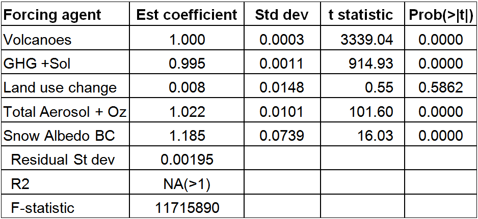 Table 2. Results from regressing all Historical forcing on five forcings over 1851-2012
The regression residuals from the Table 2 regression (Figure 5) are dominated by spikes at the time of volcanic eruptions, the origin of which is unclear.
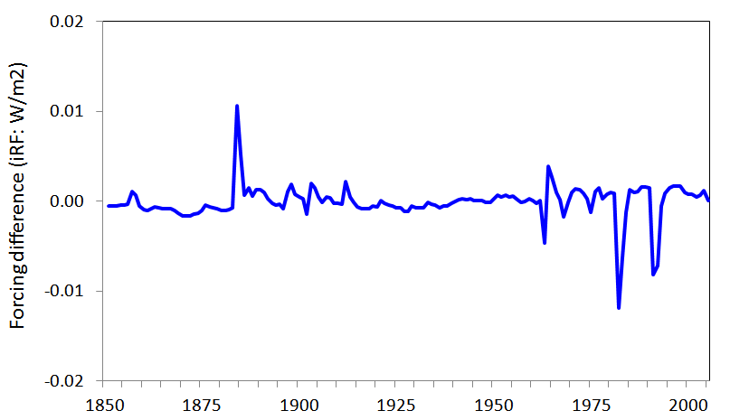 Figure 5. Residuals from regressing all Historical forcing on five forcings over 1851-2012
I am at a bit of a loss to make sense of these results. I have considered the possibility that stratospheric water vapour forcing might account for the excess of Historical forcing values over the sum of all the individual forcing values. Stratospheric water vapour forcing is not imposed or calculated separately in GISS-E2-R, but arises from the oxidation of methane.[3] It is thought to be similar to that in GISS ModelE, which was estimated as ~0.07 W/m2 in 2000 relative to 1850 – only about a third of the unexplained excess. Moreover, as the iRF estimation method involves the climate state – including water vapour and clouds – being fixed in 1850, it does not appear that stratospheric water vapour forcing would be included in Historical iRF (nor in GHG iRF).
The most logical explanation I can find for the regression results is that land use forcing was somehow inadvertently entirely omitted from the GISS-E2-R Historical simulations, not just from the archived Historical forcing values. But that would seem quite an unlikely mistake. A second possibility is that there is some flaw in my regression approach or its implementation, or that I am overlooking something obvious. Another possibility is that some interaction between forcings that detracts from linear additivity mimics subtracting Land use forcing, although what interaction might produce an appropriately shaped time profile is not obvious. Perhaps one of those explanations is more likely than that GISS slipped up. I really don’t know what the explanation is for the apparently missing Land use forcing. Hopefully GISS, who alone have all the necessary information, may be able to provide enlightenment.
Response from the authors generally
The only substantive response to date from the authors of Marvel et al. to my original article, other than regarding LU run 1, has been a comment at RealClimate by Gavin Schmidt, stating that my observation that their plotted iRF values (both for volcanoes and historical forcing) appear to be shifted by +0.29 W/m2 from the data values was misplaced, since they had used 1850–59 mean forcings as a baseline. There was no mention anywhere in Marvel et al. that this had been done. The difference is negligible except for volcanic (and hence also Historical) forcing: all other individual forcings varied very little during the 1850s from their value in 1850, the baseline year used for the data values.
The baseline used for iRF forcings is not actually relevant to my criticisms of results in Marvel et al. Since their iRF results are based on regressions over 1906–2005, with the estimated best-fit lines not constrained to pass through the zero-forcing, zero-GMST change origin, they are unaffected by the baseline used. Revising the forcing baseline alters, for volcanic and Historical forcings, the differences between Marvel’s best-fit slope and that derived from a more physically-justifiable regression basis that requires it to pass through the origin, but it does not eliminate them.
The use of a 1850–59 baseline also greatly reduces the apparent large difference between iRF and ERF volcanic forcing changes. However, that does not affect my point that the strongly positive change in low-efficacy ERF volcanic forcing to 1996–2005 depresses the TCR/ECS estimates based on Historical ERF forcing in a way that is not applicable to most observationally-based estimates. This point applies equally to the Marvel et al. iRF based estimates. The downwards bias that low volcanic forcing efficacy has on estimation of TCR and ECS from the Historical simulations would not occur if the practices used in sound observationally-based, historical period studies were followed. Such studies use analysis periods or methods that minimise the impact of volcanism, and thereby avoid bias from low volcanic efficacy.
Acknowledgements
I thank Ryan O’Donnell for the code used to produce the World projection plots.
[1] Kate Marvel, Gavin A. Schmidt, Ron L. Miller and Larissa S. Nazarenko, et al.: Implications for climate sensitivity from the response to individual forcings. Nature Climate Change DOI: 10.1038/NCLIMATE2888. The paper is pay-walled, but the Supplementary Information (SI) is not.
[2] Miller, R. L. et al. CMIP5 historical simulations (1850_2012) with GISS ModelE2. J. Adv. Model. Earth Syst. 6, 441_477 (2014). Open access.
[3] According to Miller et al. 2014, stratospheric water vapour is augmented according to the surface methane concentration, with a prescribed 2 year lag. Calculation of the forcing due to oxidation of methane is complicated, because several years elapse before the water vapour originating as surface methane circulates throughout the stratosphere.
Update 23 January 2016
I have just discovered (from Chandler et al 2013) that there was an error in the ocean model in the version of GISS-E2-R used to run the CMIP5 simulations. The single forcing simulations were part of the CMIP5 design, although it is possible that some or all of them were run after the correction was implemented.
Chandler et al write:
” We discuss two versions of the Pliocene and Preindustrial simulations because one set of simulations includes a post-CMIP5 correction to the model’s Gent-McWilliams ocean mixing scheme that has a substantial impact on the results – and offers a substantial improvement, correcting some serious problems with the GISS ModelE2-R ocean.”
explaining the problem as follows:
“the simulations described here as “GM-CORR” utilise a correction to the Gent- McWilliams parameterisation in the ocean component of the coupled climate model. In prior implementations of the mesoscale mixing parameterisation in GISS ModelE, which like many ocean models uses a unified Redi/GM scheme (Redi, 1982; Gent and McWilliams, 1990; Gent et al., 1995; Visbeck et al., 1997), a miscalculation in the isopycnal slopes led to spurious heat fluxes across the neutral surfaces, resulting in an ocean interior generally too warm, but with southern high latitudes that were too cold. A correction to resolve the problem was made for this study, and it will also be employed in all subsequent versions of ModelE2-R going forward.”
Interestingly, they also write:
“One of the most significant differences of the Pliocene GM CORR simulations, compared with those of the uncorrected model, is the characteristic of the meridional overturning in the Atlantic Ocean. In GM UNCOR the Atlantic Meridional Overturning Circulation (AMOC) collapsed and did not recover, something that was expected to be related to problems with the ocean mixing scheme. Although we hesitate to state that this is a clear improvement (little direct evidence from observations), it seems likely that the collapsed AMOC in the previous simulation was erroneous.”
It occurs to me to wonder whether this error in the GISS-E2-R ocean mixing parameterisation may account for its behaviour in Land use change run 1. It looks like something goes seriously wrong with the AMOC in the middle of the 20th century in that run, with no subsequent recovery evident. I have been unable to ascertain as yet whether that simulation was run using the uncorrected or the corrected ocean module code.
Additional reference: Chandler M A et al, 2013. Simulations of the mid-Pliocene Warm Period using two versions of the NASA/GISS ModelE2-R coupled model. Geosci Model Dev. 6, 517–531 (Open access)
Update 31 January 2016
I have now uploaded GMST and top of atmosphere radiative imbalance data from 1850 on for the GISS-E2-R runs used in Marvel et al. The data used by Marvel et al, available on the GISS website, omitted the first 50 years of simulations in the case of the GMST data, and gave ocean heat content rather than the appropriate, approximately 16% larger, TOA radiative imbalance data .


126 Comments
Am I understanding this correctly? Marvel et al. compared real world data against a computer simulation and concluded that the real data was incorrect?
Bob Carter
I think it is halfway correct. What they mean is that the real data doesn`t give the right picture of the global warming. There is some kind of latent heating that does not show up because of forcings that cool the earth. The CO2 with feedbacks does not show its right effect. The air temperatures should have been higher. These people believe that anthropogenetic part of warming since 1950 is more than 15% higher than temperature records show. So I think that all the work they lay down in modeling TCR and ECS, is to find some proof for their beliefs.
And I think that all the forcing estimates are strange. Sometime they have a great belief in effects of volcanoes, without pointing out that volcano activity ha been low for over 150 years. Sometimes they believe in aerosol effects, even if the amount of smoke and gas perhaps has decreased. Ozone can have warming and cooling effects. An now they come up with land use. It is as if they are grasping whatever explanation that can suit them. The estimates vary. When it come to the real world I think that these forcings are much smaller than is assumed.
From the discussion on RealClimate
“Todd Friesen says:
Question for Gavin or Kate (or anyone),
Based on NASA’s CMIP5 forcing model, year 2012 has a greenhouse forcing of 3.54 Wm2, ozone has 0.45 Wm2, atmospheric aerosols have -0.89 Wm2 combined direct/indirect, and land use has -0.19 Wm2, all based on iRF. If I apply the adjustments specified in the paper based on TCR to make equivalent to GHGs, then I get revised forcings of 3.54, 0.24, -1.19, and -0.68 respectively. Put it all together results in a forcing of 1.91 W/m2 out of a total of 3.78 for GHGs and Ozone. (I’ve ignored volcanoes and solar for simplicity. The ratio would be 1.79 W/m2 out of 3.66 W/m2 with the aerosol adjustments in Schmidt 2014).
Is my understanding correct that aerosols and land use then offset half of the GHG+Oz forcing? So instead of 0.9C of warming (relative to pre-industrial), we would have closer to 1.8C without them?
The AR5 chart (measuring human contribution to warming from 1950-2010) shows a much smaller aerosol offset, ie. +0.9C of warming without other anthro instead of +0.7C of warming with. The IPCC chart appears to assume no adjustments to the iRF.”
Gavin is commenting very much on the blog comments, but I cannot see that he answered this Question. Could you comment on this Nic Lewis?
What Todd Frieson wrote seems about right. I get a slightly lower figure for iRF GHG “effective” forcing (forcing x efficacy), so that over half the anthropogenic GHG + ozone forcing has been cancelled out by negative aerosol and land use change forcing.
As well as effective aerosol forcing of -1.2 W/m2 being mcuh stronger than the IPCC AR5 ERF of ~-0.7 W/m2 over 1850-2000, the land use change effective forcing of -0.7 W/m2, arsign from a very high efficacy of 3.89, seems absurd to me. It is partly due to the inclusion of LU run 1, but mainly due to the unphysical regression method used. If the regression is forced to go through the origin, LU efficacy it is much closer to one – or belwo 1 if run 1 is excluded. In AR5, the IPCC scientists thought it as likely as not that land use change actually caused warming rather than cooling.
Interesting work as always, Nic. I was taken by this line:
This is just another application of the tree-ring principle. Someone once famously said that the beauty of tree ring analysis was you get to select the temperature sensitive trees … in the same way, the modelers are always choosing the “temperature sensitive” model runs, and the rest are simply dismissed as “rogues”.
I’ve always wondered about the model runs that ended up on the cutting room floor and never made it to the movie screen …
w.
Willis, Thanks for your comment. I’m not sure how many model runs end up on the cutting room floor, once the final model version has been developed. It may be that the issue is more relevant to the discarding of model variants as unsatisfactory. Having said that, the impression I get is that models are typically tuned more by their ability to match basic features of the real climate system than by how sensitive they are. Having said that, I suspect that for models with sensitivities at the top and, maybe particularly, bottom of the model range their developers may feel that they should make changes so that their next model is more comforatbly within the model ECS range.
In the GISS-E2-R case, it seems pretty clear IMO that Land use run 1 is a rogue. No other of the > 30 single forcing runs display a difference from the mean GMST change of the remainder of the ensemble that is more than a fraction of that applying to LU run 1, and there is no physical reason for a massive ocean anomaly to develop in response to very weak land use change forcing.
niclewis said:
Nic, I’m still uncomfortable with what you call a “rogue” result. You say there is “no physical reason for a massive ocean anomaly to develop” … but clearly, the model thinks that there are very valid physical reasons for such an anomaly.
As such, saying in essence that one result is unphysical but the rest are physical seems like special pleading. Obviously, in the bizarro model world of GISS-E2-R physical constraints are such that the globe can do things totally unlike anything witnessed in the historical record.
And this means that we have no assurance that the rest of the model runs are any good. Those models are using the same obviously incorrect physics used in the “rogue” … so how can we put any weight on them?
Finally, do you have a link to the model results and the historical forcings as used in your analysis?
All the best,
w.
Willis, See this morning’s update to my post. It turns out GISS-E2-R had a mistake in its ocean module, which it seems could lead to the AMOC collapsing when it shouldn’t. That could perhaps explain what happened in LU run 1.
As you say, this does place a question mark over the reliability of other CMIP5 simulations by GISS-E2-R. It would in fact be fairly obvious if a similar ocean instability to that in LU run 1 had occurred, and there seems no trace of it having done so in any other historical period run.
In any event, Marvel use the single forcing runs to appraise how TCR and ECS estimated from observations over the historical period compare with actual, CO2 forced, TCR and ECS. Even if it is physically conceivable that a massive ocean anomaly might have developed if the real climate system had been forced by land use change, it is evident that in reality no such thing happened. Accordingly, it is not appropriate to include a run in which it did occur.
Links to the model results and historical forcing data are provided in my original post. Those are global only data. The raw temperature (tas) data is available in the CMIP5 archive; the raw files are a sizeable set of data. I’ve not processed all of the data on a gridded basis, but if you want particular tas or TOA radiative imbalance data email me and I’ll see if I can help.
Nic, thanks for your reply. You say:
I must point out again the cutting room floor. Surely the 3-5 simulations submitted to CMIP5 are not the totality of all of the GISS-E2-R model runs. And I have to assume that there is some selection process that goes on regarding what each institution submits to CMIP5.
All the best to you,
w.
Wouldn’t the more appropriate response be for any model that displays any rogue runs ever to itself end up on the cutting room floor?
If we are talking being removed from the set of ‘policy-ready models’ giving trusted estimates of sensitivity I tend to agree. But there are other uses of models in advancing understanding.
Um… no. Tons of useful models can produce unrealistic results if something goes wrong. It’s actually part of the process of some model design, where the modeler will run the model and look for unrealistic results so they can then better constrain parameters to avoid such. In other cases, rogue results are simply the outcome of bad luck with random walks.
A model which produces rogue results 1% of the time because of randomness in the model not being constrained enough can still be very useful. Especially since problems like this can be limited to one part of the model while having little to no affect on the rest. Why scrap everything because of that?
Discarding runs that dont seem reasonable is an ex post selection of data, this practice gives the impression that the results of the set of runs is more tightly grouped than is actually the case.
At a minimum, there should be an established protocol for discarding individual runs, one established before they are generated; these discarded runs should be included for examination, and the reasons for their removal from the set before further analysis should be discussed.
100% agree with that David. This should be basic to climate openness, rightly understood.
Ditto. I am dismayed by the complacent disregard of the ex post use of model products. It sounds like a process of random generation of products from which are selected the ones which best suit the aims of the investigator.
A couple of thoughts for what its worth.
If a model is found to have errors the fact that this was discovered after it was used doesn’t mean you can’t reject the results.
Its just that you should reject all of them.
And if you do get one strange result in a small number of runs, it is a salutatory reminder of the problems of drawing inferences from small samples. The error bars on any reported results must reflect this.
David,
The result of a model isn’t “data”. Just some numbers pertaining to the model.
Correct, Jeff, in the proper sense it is not data, only product of the model.
But it is treated as data. How often do we hear “the models tell us that…”
Were this sort of confusion not the basis of international policy decisions, it would be amusing.
And now we see that the products of GCM’s are sifted and selected, and unwanted “data” is discarded.
Jeff…data is information, the plural of datum.
I believe what you mean to write is something along the lies of;
“model output isn’t direct observational data” or something like that.
model output is data, most assuredly…it is information about the models’ outputs,and performance.
David,
Fair enough but how do you distinguish between data that carries useful information and noise?
We have no way of knowing if the output from a model is useful information for anyone beyond the modeller. Calling it data adds credence to something that may only be brightly packaged numbers.
Consider how they average together the output data from numerous models to create an ensemble result. This sounds a lot better than averaging together the brightly packaged numbers from numerous models to create sparkly number picture.
Jeff:
You make a good point, and I would only add that if one cant articulate a means of differentiating between a model run that is useful, and one that contributes only noise BEFORE one conducts the runs, then one acknowledges that there is no way to tell the difference, other than “this looks too undesirable to include”….
As for averages of the outputs from different numbers of runs of different models, this enterprise in not supported by any reputable statistician; the multi model mean is a bankrupt concept.
And yes, the creation of a “sparkly number picture” is quackery at its finest, IMO.
“I have now heard back from Ron Miller to the effect that, although LU run 1 indicates greater cooling, he doesn’t regard the run as pathological and can’t see any reason to treat it differently, and that they don’t have any current plans to rerun this simulation”
####
Do Marvel et al imagine that the rest of science will join them in ignoring that peculiar, dark blue blotch in the North Atlantic?
Land usage forcing, as per their model run.
Great work, Nic, thank you. I am not a climatologist, but your analysis confirms my suspicion that we know very little about climate. My conclusion may change when I see a reliable 100-hour weather forecast.
But this ongoing climatology research does have a very reliable course, and can be easily forecast. Data that indicates previous over-estimation of anthropogenic GHG forcings must have some other explanation.
Good one and very true, it would be sad if it wasn’t making most of us poorer and killing some of us.
On 18 January on RealClimate Sven followed up on my 8 January request for a response to Gavin Schmidt regarding Nic Lewis’ first article on Marvel et al. here at ClimateAudit:
January 8
[Response: Mostly confused, but there are a couple of points worth following up on. Should have the relevant sensitivity tests available next week. – gavin]
??
[Response: Patience grasshopper… – gavin]
Looks like an Indian “next week”….
Thanks, Paul, a very interesting point about the forcing calculation not being automated. It certainly seems less unlikely that GISS scientists might have missed out LU forcing when deriving iRF values for the All forcings case offline than when setting up the Historical simulation itself.
Your speculation about what Gavin means by “sensitivity studies” seems to me pretty likely to be the case.
Nic,
“when another single forcing run had, for unknown reasons, an unreproducable excursion in the middle of the run.”
I am astounded by this, for two reasons: 1) if the model can sometimes ‘go off the rails’ for no apparent reason, then it seems unlikely the model is a reasonable representation of the Earth’s climate, and 2) at an absolute minimum, there should be a careful investigation into the stability of model behavior, with lots of runs, so that the probability of a ‘crazy’ run is at least known. If crazy runs are going to be ignored, then some defensible criteria have to be used….. and that shouldn’t be ‘we didn’t like that run’. Were anomalous runs discarded when the CMIP5 ensemble was being developed? We don’t know, but maybe Gavin does.
Suppose the vagrant excursion occurs in 2027 and causes the rejection of the only “accurate” (must be a better word) run ever?
Maybe less sci-fi, how often are runs rejected because they appear to predict badly but are ok in known territory?
Since none one has stated the obvious, I may as well.
Nice Lewis:
I drew this finding to the attention of Ron Miller of GISS, one of the Marvel et al. authors, last week, asking whether he had any explanation and enquiring whether the simulation might be rerun, as GISS had done when another single forcing run had, for unknown reasons, an unreproducable excursion in the middle of the run. I have now heard back from Ron Miller to the effect that, although LU run 1 indicates greater cooling, he doesn’t regard the run as pathological and can’t see any reason to treat it differently, and that they don’t have any current plans to rerun this simulation.
###
This response by Miller is full of implications. What sort of criteria do they adhere to, it must be asked.
Nic –
A mainstay of the skeptics argument at various places is that the last 18 years of satellite observations are wildly less than the modelled (IPCC) scenarios. Yet you and Judith Curry (and others) don’t seem to have a problem with the so-called disconnect. Is the truth that scenarios and observation datasets have enough internal uncertainty that ALL of them are equally valid at this time?
There is something I call Computational Reality vs Representational Reality. Models reflect Computational – the results are exactly what they should be based on the assumptions and data input. You can trust them to produce identical results 100% of the time. Representational Reality is what is actually going on in the world – the sort of knowledge that God might have. The public and politicians conflate the two, but to get Computational to actually mimic Representational is really, really hard and nobody thinks we are certain that has happened yet.
The authors of Marvel et al therefore will vehemently disagree with you here and – in the Computational Reality way – will be correct. GISS2015, HadCruT4, RSS/UAH are all correct in their own way, and equally supportable but none of them are – even by the authors – known to be NECESSARILY correct, only a decent guess.
Is that what you and Curry think?
douglas,
The models don’t produce identical results every time – they have internal variability. But unlike in the real climate system, one can reduce the effects of internal variability in models by performing multiple runs with the same inputs, and averaging the results.
I’m not sure whether ~15 years is a long enough period to conclude that the model projections are seriously out of line with reality, given the existence of not very well quantified decadal and multidecadal internal variability in the real climate system. The 18 year figure arises from the very strong 1997/8 El Nino, and doesn’t really provide an unbiased comparison with models (although, in a year’s time, using the 1998 to 2016 period may do so, given the present strong El Nino).
I think it is better to compare the full satellite record, which is now 37 years long, with model simulations. Doing so shows that the models have warmed much more strongly, with a few exceptions. And for estimating the sensitivity of the climate system to GHG and other forcings, using the full length of the instrumental record (from 1850 or 1860) seems best to me; many other scientists have also made this choice.
Nic,
Thanks for your reply. Understanding is more nuanced, as I suspected.. Strong, rigid positions on both sides are not really justified, either, once uncertainty issues are out in the open.
Nobody can hold to the claim that McDonald’s or Burger King make a “perfect” burger, once they admit they are talking about fast-food.
The claim that AGW caused the warming prior to 1950 is junk food not even the IPCC will touch.
Yes mpainter, that’s true.
Of course, we’ve seen some of the warmer data in the distance past flattened over time.
Can Miller, or any among Marvel, et al., explicitly state the parameters they use to exclude rogue/pathological results?
Without explicit ranges for identifying rogue runs, how would they know whether a particular run was actually a one-in-a-million outlier? Is it based on more than just a gut feeling?
If LU run #1 is not, in fact, an extreme outlier I would expect something like it to show up with similar frequency in, say 20 (or 100) simulation runs. If computational burdens make high-volume simulation runs impractical, wouldn’t you expect the authors to have already tested sensitivity ranges, prior to publication?
It appears to me that, between the Nic and Paul observations posted here, there might well be an omission by the Marvel authors or at the very least an explanation from them about these findings/observations is in order.
If an author of that paper sees no problem with that LU run not being an outlier one would have to put that occurrence onto expected variation in multiple model runs. I wonder what a higher number of multiple runs model runs would have produced. It also makes me curious enough to go back and use my downloaded Marvel data to determine by a Monte Carlo approach the confidence intervals for the individual and combined forcings using various forcing baselines.
Nic, do the coefficients in your multiple regressions being close to 1 have any implications for efficacies being close to 1?
Ken, No, I’m just regressing the Historical (All-forcings) forcing time series on the forcing time series for the constituent individual forcings.If they have been correctly included in Historical forcing, the coefficients should contain one within their uncertainty ranges, as they do except for land use forcing where they are consistent with zero.
For “internal variability”, given that we’re talking about computer code, one ought to substitute the words “randomly generated values”, yes?
If there were no randomly generated values, then clearly the output of each run would be identical.
I’d like to understand the justification for the introduction of randomly generated numbers into the model … for this tells me that they are substituting a lack of real world data.
“we’re guessing the data” doesn’t seem like a great criteria for apprehending some form of true knowledge.
I beleive there are no randomly generated values as such in current computer models. The internal dynamics of the model generate internal fluctuations; when the model is run for a long time in the preindustrial control run all state variables fluctuate about quaasi-equilibrium values. The forced runs are spawned from (branched off) the piControl runs at different point – 20 years apart in the case of GISS-E2-R. So they do not start from quite identical positions. Those starting differences will change as the forced runs proceed.
One would therefore not expect the output of each run to be quite the same. But they should be similar, the more so the period that they are compared over. And they are: the standard deviation of the mean global temperature over the last 50 years of the historical period for the runs making up the simulation ensemble for each single forcing is 0.02 C or less. Except for the land use change runs, where it is 0.08 C. Excluding outlier LU run 1, that standard deviation drops to 0.01 C.
Nic -“when the model is run for a long time in the preindustrial control run all state variables fluctuate about quaasi-equilibrium values.”
What causes the steady states? I mean is it calculations based on physics or just range limits in the software?
jinghis – the quasi steady states result from calculations that reflect the physics involved, in some cases directly and otherwise using parameterised approximations. There are no range limits in the software, I think.
Can someone tell me what “land use” factors contribute to “cooling”?
Normally it’s been said that our urbanization efforts and poorer desecration of arable land has resulted in an enhancing of warming.
If there’s a way we’re using the land such that it causes more cooling, particularly a pronounced/prolonged cooling, then what’s to say we just keep doing more of that..?
The primary reason is an increase in albedo when forest etc. is cleared for farming. The refelction of more sunlight causes cooling. Irrigation, and effects of forest removal on precipitation and wind, also affect local climate.
Is it known to what extent GISS models still rely upon the original Hansen 1998 estimates for increased albedo from LU changes?
Hansen 1998 estimated “global land-use climate forcing as -0.2W/m^2 with uncertainty 0.2 W/m^2.” Hansen’s analysis was limited by some fairly crude initial assumptions, albeit justifiable given the state of knowledge 20 years ago. Have subsequent studies confirmed, or just continued to assume, that Hansen’s original estimates accurately reflect global conditions?
LU forcing in GISS-E2-R reaches -0.19 W/m2 during the 1980s, relative to 1850, and stays constant until 2012. IPCC AR5 estimated LU albedo forcing as -0.15 W/m2 from 1750 to 2011, and at -0.11 W/m2 from 1850 to 2011. So the GISS estimate is rather higher than the IPCC estimate, which should have taken all relevant subsequent studies into consideration.
It is interesting to me that they have low confidence in the sign, to say nothing of the magnitude, of the net impact from global changes in land use.
From the WG-1 Technical Summary:
Thank you again for this illuminating analysis.
Nic,
Baffin Island is a critical – perhaps the most critical – area of incipient glaciation in low summer insolation at high NH latitudes (Milankowitch). See for example the recent discussion of incipient glaciation by Ganopolski et al (2016) (url)
According to the assumptions of their model, they observed incipient glaciation in Baffin Island in one of four model runs at 280 ppm CO2 (and all runs at 240 ppm CO2.)
The cold area in GISS Run 1 is contiguous to the area of incipient glaciation in the Ganopolski model runs, that occurred in some, but not all, runs. Question: maybe Run 1 triggered Baffin Island glaciation, whereas the other runs didn’t.
BTW whereas Ganopolski et al asserted that there is no evidence of actual incipient glaciation, there was substantial expansion of Baffin Island glaciers during the Little Ice Age, expansion which seems to accord with a Ganopolski case much more than they acknowledge. Also in Iceland in the 19th century, ice-rafted debris (IRD), indicating expanded glaciers, occurred for the first time since the LGM.
In other words, it may very well be that the cold Run 1 is not necessarily rogue, but an incipient glaciation case. One would have to check other details of the GISS run to verify.
Steve,
A very interesting point. But the land use change forcing is very small (a fraction of that in the aerosol single forcing runs, and equivalent to a reduction on only ~7 ppm CO2 at the time the anomaly occurred). In fact, the aerosol forcing only runs show signs of exactly the opposite effects, with the same ocean patch south of Greenland warming and the opposite pattern of changes off Antarctica. So it would seem a bit surprising if land use forcing were enough to itself initiate glaciation.
Maybe it is more likely that LU forcing had enough of an effect in the version of GISS-E2-R used (at least for other CMIP5 runs), with the faulty ocean mixing scheme? Also, Chandler say that GISS-E2-R has a regional cool bias in the upper mid-latitude Atlantic, in its preindustrial control run. Whatever the cause, it looks to me as if there is a change in the AMOC involved.
As I wrote earlier, whether or not LU run 1 is strictly a rogue, it seems to me that there is a good case for excluding it since we know the real world climate system did not behave like this during the 20th century.
Has anyone seen the most recent Ganopolski paper that got a big PR push?
“Human-made climate change suppresses the next ice age”
https://www.pik-potsdam.de/news/press-releases/human-made-climate-change-suppresses-the-next-ice-age
Oh, my mistake! I didn’t notice the url link in your comment. Thanks for the link!
I can just agree with Marvel in one thing (from her blog):
“The climate’s sensitivity is hard to nail down, but mine is pretty high.”
Well, that it is “pretty” high is an understatement.
When I see some evidence that the (software) models were written by (software) experts and have been developed using industry standard best practices, then I will start taking them a bit more seriously. Until then, they are about as useful as an uncalibrated piece of lab equipment.
Nic,
Re your latest update, Gavin Schmidt noted the heat transport problem in the Russel ocean model in a paper published in March 2014. (http://onlinelibrary.wiley.com/doi/10.1002/2013MS000265/full). It looks like it had not been fixed up to that time.
The Miller et al paper was published in June 2014. (http://onlinelibrary.wiley.com/doi/10.1002/2013MS000266/full). As far as I can tell, the Miller paper mentions the existence of the problem but no correction.
I think a polite question to the authors is justified. Given a free choice of GCMs, I would not choose to use OHC data from a model with a known ocean heat transport problem. However, it is possible that a corrigendum was issued for the GISS-E2-R results, and the data accessible via the CMIP5 portals updated. If so, it would be good to have a pointer to it.
Paul,
The Schmidt and Miller papers were submitted at the same time, so I would expect them both to reflect the same position regrading correction or not of the ocean problem in GISS-E2-R. I can find no mention of the problem in the Marvel paper, nor in a paper submitted over a year later about the climate change in GISS ModelE2 under RCP scenarios (http://onlinelibrary.wiley.com/doi/10.1002/2014MS000403/full 2015).
I cannot find signs of any corrigendum for GISS-E2-R results. It is conceivable that in practice the effects of the ocean problem were small, at least in all the main simulation runs. I have redownloaded CMIP5 r1i1p1 tas netCDF files for the GISS-E2-R Historical simulation. They have the same file date (25 March 2011) as those current at the AR5 March 2013 cutoff date.
Nic,
Do you happen to know if and how AIE was included in Miller’s “All forcings together” values for Fi? This would not automatically appear in the instantaneous net flux perturbation and would need to be added in either by using the parameterisation algorithm in GISS-E2-NINT or by adding in the values calculated from the single-forcing case or other. I can find no reference in Miller to any such calculation, but I may have missed it. It must of course be added in for any efficacy calculation to make sense.
Paul,
I don’t know for certain that AIE was included in Miller’s iRF (Fi) “All forcings together values”, but I have assumed that it was. Miller says the that magnitude of the AIE is tuned using an empirical relation between low cloud cover and the logarithm of aerosol number concentration, and that in 2000 the instantaneous AIE at the tropopause is -0.67 W/m2. A value for AIE iRF could have been calculated by perturbing the 1850 cloud field used when when computing iRF, although there is no mention of doing so in Miller et al.
Wouldn’t adding in values calculated in the single forcing case simply push the question of measuring an iRF for AIE back to that simulation?
As you will know, aerosol indirect effect should not really appear in iRF at all, since adjustments by clouds are not instantaneous; Hansen 2005 did not show any iRF value for it. But there is quite a lot of discussion in Miller et al about aerosol forcing in Miller et al, which would all be wrong if the AIE had not been included in their All forcings together measure, so Ron Miller seems happy that it was included. And my multiple regression results certainly support AIE forcing having been included.
Thanks Nic,
I agree that your multiple regression results support AIE forcing having been included – in some guise. And certainly, what was done in Marvel et al would make no sense if it had not been included, so no doubt the co-authors believe that it is already included.
What was going through my mind was the difficulty of assigning any equivalent Fi value to AIE for the historical run. Miller makes it clear that he uses pre-industrial climate for the evaluation of Fi values. This does not require any simulation. It just requires activating all of the forcing agents, turning on the radiative code at annual intervals and recording the net flux change at the predefined tropopause. Because there is no atmospheric simulation involved, AIE does not manifest itself in this calculation. Strictly speaking, it is not a forcing at all, but a fast feedback which is unique to tropospheric aerosols. Because it is unique to this particular driver, as opposed to being a temperature-dependent feedback common to all forcing drivers, it must be treated as a quasi-forcing in order to permit intelligent comparison with other forcings in general and with CO2 forcing in particular.
Hansen’s algorithm for AIE (which I described as “the parameterisation algorithm in GISS-E2-NINT” and which you call an “empirical relation”) does permit the indirect effect to be converted into an equivalent forcing. So what I suspect was done was that the algorithm was switched on together with the radiative code at each time period. The problem with this is that the equivalent forcing value is strongly dependent on climate (and particularly cloud cover) at the time the algorithm is calculating. From the above process for abstracting Fi values, cloud cover is fixed at pre-industrial level. The difference in calculated values may be substantial (see Hansen 2005) between fixing the cloud cover and allowing it to vary (as it did in the actual historic run simulations). If this is what Miller did, then he should be able to isolate very simply the AIE forcing from the historic run and confirm that it was identical to the single-forcing case abstraction of AIE on the same basis of unchanging climate state. That then allows a more definitive statement to be made on the difference between the calculated/assumed AIE in the historic run and the “true” AIE which was based on the successively updated climate state and which should be, I believe, significantly more negative.
(The alternative to which I referred involves analysis of the single-forcing run simulation rather than the abstraction of Fi values from the same, but I suspect it is not very relevant. The indirect forcing can be abstracted by de-convolution of the temperature and net flux data since there is only one known direct forcing which is changing.)
I have left a question on realclimate hoping for some clarification of what was actually done.
Here is a copy of the comment I left on RealClimate.
Gavin,
I would be very grateful if you could respond to the following three questions.
1) Do you have available CO2 benchmarking data for GISS-E2-R, specifically, estimates of Fi, Fa and ERF for a range of concentrations? If not, more specifically, are you going to support or modify the Fi value of 4.1 which appears in Marvel et al?
2) Can you please advise if and how AIE forcing was included in Miller’s “All forcing together” Fi values for the 20th century historic run?
3) Can you confirm that the temperature and net flux data for GISS-E2-R, available via the CMIP5 portals and KNMI Climate Explorer are based on a model corrected to fix the ocean heat transport problem which you identified in the Russell ocean model in your 2014 paper?
Many Thanks
If an algorithm can produce results that are clearly “rogue” then I would imagine it can produce results that are “partially rogue” as well. As a software developer myself, I think this creates a situation where a “bug” becomes a subjective decision. In order to make the determination more objective one would need to define “rogue” more clearly.
It’s sort of a catch 22 when you design code whose purpose is to find out if anomalies will occur in that your code needs to be free to create anomalies which could just as easily be coding/logic errors. I would think code of this type would always have to have an independent verification method to check predicted anomalies, (such as reviewing the physical plausibility of the processes involved). In other words, I think these models should be used to present questions, not answers.
As striking as LU run 1 is (fig. 4) it looks like it has half the scale bars of fig. 1 (runs 2-5) – -2.5 to +2.5 vs. -5 to +5.
Is this just a matter of the legend not being updated…?
Fig.4 has the same scale as Fig.3, not as Fig 2 (which I assume is what you meant by Fig.1). A version with a 5 C scale is here.
Yes, sorry – fig. 2 is what I meant. What I was pointing out was that the scale should be the same on all the ‘single run’ figures.
Thank you for the link to the figure with the extended scale. This seems to show that a -5 anomaly occurs in the north Atlantic, not just a -2.5 one as per fig. 4. Of course, the blues do not look as dramatic with the colour ramp stretched.
Going back to Nic’s pdf critique of Marvel and then rereading Marvel, the criticisms that Nic makes of this paper become clearer to me. More importantly in addressing the quality of this paper it is the accumulation of problems that Nic sees in this paper. It is that accumulation and not necessarily a single problem pointed out that is the important to judging the validity of the results/conclusions of this paper.
What I have seen in the past with criticism of climate science papers from these blogs, like Climate Audit, is that an author or defender of the paper will clear up or attempt to clear up a single point and fail to answer/acknowledge the many problems. We who are critical sometimes concentrate on a single issue without continuing to point to the multitude of issues. I would hope that the Marvel authors will address all of Nic’s criticisms, but if they do not that might well say something also.
Interesting also that the efficacy measures made by Marvel could in some sense and context be construed as factors required to bring the model sensitivity more in line with the empirical results using mostly observed data and that obtains lower sensitivities. Going forward and without knowing the origin for the need of the efficacy measures significantly different than unity, one might well conclude that prediction of future temperature increases from AGW would be the same with or without the efficacy measure.
The Marvel paper gets around this thought by talking about the “accident of history” and implying that the efficacy measure is very much unique to the recent climate conditions and pointing to the efficacy measure different than unity being related to the non uniformity in the x,y and z directions of the global atmosphere of the negatively forcing agents.
It reminded me of the thought process of some climate scientists implying rather strongly that the divergence of proxy responses in recent years must be related to AGW – otherwise, of course, without an explanation we have to seriously question the proxy responses in past times to temperature never minding that the selection process in most of these temperature reconstructions makes the process flawed from the start.
As a (now retired) professional programmer, I’m astonished that anyone believes that:
* Large, opaque computer programs work
* Large, opaque computer programs meet their specifications (if any)
* Programs (and their specifications) accurately represent anything as large, complex and poorly understood as world climate
* Programs (and their specifications) accurately embody the Physics that we do understand like Conservation of Mass, Navier-Stokes Equations and on and on
* Programs (and their specifications) should ever serve as a basis for public policies that could result in impoverishment, starvation etc.
Several of the computer program output anomalies mentioned by Dr Lewis smell to my practiced nose like program bugs.
Regards,
Bill Drissel
Frisco, TX
Nic, I have been attempting to find the data for the 6 multiple model runs used to determine the ERF for the individual forcing agents in Marvel. I find only 1 set of data for these forcings for ERF. I was under the impression that ERF and iRF data were both taken from multiple runs.
Ken, Miller says that iRF is determined by measuring th eradiative imbalance in the 1850 climate state as it was before perturbation by any forcing, but with the relevant forcing(s) imposed. That would give the same result for all runs, as the climate state has not changed from preindustial. So it would just be computed once, I think.
For ERF the SST is fixed but the atmosphere is free to evolve. In principle multiple runs would be desirable, but as equilibrium is reached quickly with fixed SST it looks aas if they have instead, for each forcing, averaged across 3 decades from the same run. And I don’t think they have archived the fixed SST runs involved – they don’t seem to be in the CMIP5 archive.
Nic, I was not clear about my confusion with the data used for ERF and iRF approaches to efficacy determinations in Marvel, but I think I may now have it figured out – if you can verify that my understanding is correct.
All the data required for the iRF approach was available to me in the form of annual GMST and OHC for all the model runs and for all the individual forcing agents and the one set of annual Fi data for each of the forcing agents from Miller (2014).
My confusion was with the ERF approach and the source of the GMST and OHC data required to go with the one set of ERF data. As you note there are ERF data for 3 different decades for all the forcing agents from a single model run. It would have been nice to have data for multiple runs, but it is now my understanding that the same GMST and OHC data used in the the iRF approach must have been used in the ERF approach by using the average delta T and trends for OHC from the decade 1996-2005. That gets me to the multiple runs for the ERF approach and the method used in Marvel to obtain uncertainty for both the iRF and ERF approaches to determining efficacy. Is this understanding correct?
I plan to analyze the data using Singular Spectrum Analysis and other analysis approaches.
Ken, Yes, you should use all the same separate run GMST and OHC data with the one set of averaged-over-3-decades ERF data. But as there is only ERF data for year 2000 forcing, efficacies have to be calculated from quotients rather than being able to use regression. Marvel’s regression-with-intercept-over 1906-2005 method is unsatisfactory in any case.
You might get better results using data starting in 1850 (or 1851 – there is a slight jump) rather than 1900, and TOA radiative imbalance rather than ocean heat content data, for your analysis. I’ll try to add such data to that which I have already provided (at https://niclewis.wordpress.com/appraising-marvel-et-al-implications-of-forcing-efficacies-for-climate-sensitivity-estimates/)
I have left another comment on RealClimate for Gavin to mull over (awaiting moderation – copy below), while he is, I trust, assiduously working in the background to answer the previous questions which I have left.
Gavin,
You wrote:-
“Dropping outliers just because they don’t agree with your preconceived ideas is a classical error in statistics – it’s much better to use the spread as a measure of the uncertainty. – Gavin”
Another classical error in statistics is to attribute the error associated with one property to the wrong variable.
Work by the RNMI, Sybren Drijfhout et al 2015, (http://www.pnas.org/content/112/43/E5777.abstract) confirms that GISS-E2-R has the capacity for abrupt climate change in the form of (inter alia) the local collapse of convection in the North Atlantic.
In this instance, if the results of the “rogue run” in the single-forcing LU cases are due to the abrupt collapse of N Atlantic convection, as seems increasingly likely from the data, then the dramatically different temperature response in the rogue run has nothing whatsoever to do with the uncertainty in transient efficacy of LU forcing. The inclusion of the run leads quite simply to an erroneously inflated calculation of the mean transient efficacy for LU, and a misleading confounding of the uncertainty associated with the GCM’s internal mechanics with the uncertainty in LU transient efficacy.
Ultimately, the Marvel et al paper seeks to argue that sensitivities estimated from actual observational data are biased low on the grounds that GISS-E2-R over the historic period is responding to an overall low weighted average forcing efficacy. It then seeks to extend the conclusions drawn from the model to realworld observational studies. Since, we know from the real observational data that there was not a collapse of N Atlantic convection, then quite apart from other methodological questions, the inclusion of this run for the LU calculation is impossible to justify, and, on its own, is sufficiently large in its impact to bring the study results into question.
Applying the same logic, any of the 20th Century History runs which exhibited similar abrupt shifts (Southern Ocean sea-ice, Tibetan plateau snow melt and N Atlantic convection) which were not observed in the realworld, should have also been excluded from the ensemble mean for Marvel et al to have any hope of credibly extending inferences to realworld observational data – even if we suspend disbelief with respect to other problems associated with data, methods and relevance.
Paul,
Another good question for Gavin.
But I think you are unlikely to get a reply to ANY substantive question about Marvel et al at Real Climate, unless it is a ‘question’ which lends support to the conclusions of Marvel, or so silly a question that Gavin can just poke fun. Gavin is not going to entertain substantive doubts about Marvel, any more than Eric Steig was willing to entertain substantive doubts about continent-wide Antarctic warming, even after O’Donnell et al was published. The point of Marvel et al is to raise doubts (in a high profile publication!) about the veracity of the many low empirical estimates of sensitivity, so that those empirical estimates can be waved away when public energy policy is discussed. Marvel et al is just ammunition in the climate wars; IMO, its quality and accuracy do matter at all to the authors.
I think your last sentence left out the word “not”, and with that I can say ditto to your comment. Marvel et al are now at the point where to engage the issue any further only exposes (and emphasizes) the hollowness of their whole position, faulty models and all.
mpainter,
Yes, I left out the word ‘not’.
Paul,
Gavin has replied to your comment. He completely rejects your suggestion that the single very strange land use run is not representative, and so should not be included in the analysis. He also challenges you to look at the level of variance in all 200 runs of the study and do your own analysis. Seems to me that a very reasonable argument can be made about the statistical validity of any 5 run ensemble that includes a single ‘strange’ run if you know the variability of a much larger group (eg Gavin’s 200 runs).
Is Gavin admitting something there? “the basic result which that the historical runs don’t have the same forcing/response pattern as the response to CO2 alone”
Paul K,
After thinking a bit more about Gavin’s reply, it seems to me it should be possible to show the single ‘strange’ run for land use (run #1 from figure 5 in Nic’s original post) is likely to be a statistical fluke related to model behavior, and not at all representative of the actual effect of land use. If you calculate the slope of each of the five land use runs, and then calculate an unbiased estimate of the standard deviation of the slopes from runs #2 through #5, then the slope of run #1 may very well be outside the 95% inclusive probability window. That is, run #1 is unlikely to be a member of the same normally distributed sample population as runs #2 through #5, and so is more likely due to an unrelated effect which just was not present in the other LU runs. A drastic (and wildly unrealistic!) change in North Atlantic ocean temperature would of course be a plausible “unrelated effect”.
Nic,
Can you point to where the data used to generate figure 5 in your original post is located?
steve, Interesting idea. The data is available in a spreadsheet via the link given at the end of my original post: https://niclewis.wordpress.com/appraising-marvel-et-al-implications-of-forcing-efficacies-for-climate-sensitivity-estimates/ . The graph is in the tas sheet at cell ~ BN100. Right click in the graph and choose ‘Select data’ to see which ranges the data comes from.
Nic,
Thanks. The slope statistics are:
Relative slope
R1 -0.0369
R2 -0.0066
R3 -0.0144
R4 -0.0098
R5 -0.0085
Mean (2-5) -0.00982
Std deviation (2-5) 0.00332
R1 Standard Deviations from the mean: 8.15
The estimate of the standard deviation is the unbiased estimate (using (n-1) in the denominator).
So it seems to me unlikely that R1 is in the same population as R2 to R5, especially in light of the peculiar pattern of cooling in Run #1. Of course, Gavin (in his best Steigian imitation) is going to discount any slope analysis as irrelevant, or will insist, ignoring any reasonable interpretation of the actual data, that the correct analysis is to include all 5 runs in the estimate of the mean and standard deviation for the slopes. In this case, the statistics become:
Rel slope
R1 -0.0369
R2 -0.0066
R3 -0.0144
R4 -0.0098
R5 -0.0085
Mean -0.01524
Std deviation 0.0124
R1 Standard Deviations from the mean: 1.74
Which puts R1 just inside of the credible range….. if you choose to ignore the bizarre pattern of cooling in the North Atlantic, which is absolutely not a credible response to a tiny forcing from land use change. But such things seem to pass as credible when the results match the desire outcome.
Reblogged this on I Didn't Ask To Be a Blog.
My apologies if these graphs that I have linked below have been displayed by someone previously. The graphs represent the regression of the Marvel GMST versus forcings and plotted on a yearly basis. For each forcing agent I have graphed together the Ensemble mean and the 5 model runs. I think these representations paint a different picture than using decadal averages. Notice that using different parts of the forcing range would give very different trends. Where the forcing is changing with time in a trending manner then one could state that the trends would be very different depending on the decade used.
I have also calculated the trend statistics from the yearly results graphed in the links, and while the p.values can be impressive over the range of forcing, as noted above the trends calculated within parts of the range can change dramatically. I have not yet applied the auto correlation (ar1) to simulations to determine the confidence intervals for these trends but when I finish I will report the results here.
That model run for land use in question is very different than the other runs not only in the trend value but in the p.value of that trend. One can use an alternative method to determine statistical differences by using the model run trend values and the confidence intervals derived from Monte Carlo simulations as described above. I have not done that yet but I would predict at this point that there would be a significant difference between the run in question – if the confidence intervals for the other land use runs are not too wide.
Link for GHG and O3:

Link for Solar and Land Use:

Link for Volcanic and Anthro Aerosol:

Ken Fritsch,
Yes, LU Run #1 is wildly different from the others. I doubt using decadal averages (like Nic did) makes much difference in the trends… Run #1 is nothing like the other four, no matter how you look at it. I think the argument needs to be made that inferring anything about the efficacy of LU forcing with Run #1 included will lead to spurious results.
BTW, I (gently) suggest that you use the same y-axis scale when comparing the trends for the five LU runs. Using different y-axis scales obscures how different Run #1 is from the others.
Steve, Marvel used decadal averages and Nic merely reported the results. Decadal averages will graphically paint a very different picture than using the individual variation in individual runs with yearly data points. The calculated confidence intervals need to use yearly data. Using decadal averages for that purpose would require some adjustments. The differing y-axis ranges were just to see if you were paying attention.
I am finishing the CI calculations and will post them here. By my methods the land use Run 1 slope trend is statistically very different than the other runs. It would appear than some model runs for the various forcing agents have slopes not significantly different than zero. Maybe we can get Gavin to argue for the validity of that happening if we had more than one realization of the earth’s climate.
Nic, I have a post in moderation that has graphs with regressions of the temperature response to 6 forcing agents from the Marvel data. It is on a yearly basis and I think shows the data in a different light than how it was presented in Marvel.
Steve: unmoderated. triggered by number of links
I should have added that the large p.values to which I refer in my moderated post should be large negative values.
In the link below is a table with my analysis details of the regression of temperature versus forcing for the 6 forcing agents. It shows the trend, 95% plus/minus confidence intervals (CIs), the intercept, the p.values for the trend and intercept unadjusted for auto correlation and the ar1 values used for adjusting the CIs for auto correlation using 10,000 Monte Carlo simulations. Notice that slope of the trend in each case can be used to ratio amongst the forcing agents to relate back to the relative efficacy values found in Marvel.
My results for some of the forcing agents is in general agreement with those from Marvel but not all. There is a large difference for anthropogenic aerosols. I used the sum of the direct and indirect aerosol values provided by Marvel and that sum when regressed against the aerosol temperature gave very good correlations with very low trend p.values. My slope values had only one forcing agent with a higher value than GHG and that was Land Use. Land Use has slope values for the 5 runs that vary greatly and the CIs for those individual runs are large but show that Run1 is very significantly different than the other runs. Run 1 also has a trend p.value that is much lower than the other runs and the intercept is significantly different.
I would judge from the large variations within the Land Use that regression iRF versus temperature for that forcing agent makes little sense. GHG and Volcanic were the only forcing agents that had CIs that were a low percentage of the slope values. Why my calculations give such relatively low values of forcing agents slopes compared to GHG (with the noted exception of Land Use) is a puzzle to me. If I have not made a mistake here it would also throw huge doubts into the use the instantaneous forcing and regressions to determine efficacy.
Ken, I agree your slope trends apart from Anthro aerosol, where I think you may have made some mistake, based on regressing on annual 1900-2005 data. Marvel used decadal data, which gives somewhat different results. If not following their method, I think there is merit in using data for the full 1850-2005 simulation runs; I’ve now uploaded that to my web pages: see the link in the update to this article, above.
The low efficacy for volcanic forcing is expected, and partly reflects the delay in GMST reponse to a forcing impulse, which matters here as volcanic forcing is impulse like. With decadal data, there is much less distortion as a result of the delay. The same applies, to an extent, to solar forcing.
Nic, your points are well taken and now I will attempt to get my head around what you state here. Would a delay in temperature response change a trend measured on an annual versus decadal basis? There would be a lag but the response would eventually be manifested in the temperature – I think. If I used the start and end points only the trend should be near the same. Obviously there are differences – as you indicate you have made the annual and decadal calculations. But is it caused by the lag effect?
I’ll have another look at my AA trend calculations. There was a good correlation and I guess that delayed my looking. I notice from my plot of temperature versus AA that if I regressed only on the lower levels of forcing I would obtain a much steeper slope and closer to the “expected” value.
Nic, I may have had a problem with the instantaneous part of the forcing in my thinking. If I am measuring temperature response to forcing for a given year and if all the forcing were to occur and was reported in that year but only part of the temperature response occurs then that year would show a lower than expected temperature. The next year I would have no forcing but a partial continuation of the temperature response and that year would have a higher than expected temperature given no forcing is reported. I was unfortunately thinking about an accummualtion of forcing and temperature responses for my starting and ending point thought. Maybe that is what Willis was thinking.
A sufficiently lagging response might even make a decadal average of instantaneous forcing a poor method of determining efficacy. Even an event that forces in one decade and is mostly measured in another could create a problem. Conclusion: Use ERF.
I found my error with AA and the revised data and graph are in the link below. Considering the CIs for the GHG and AA the mean trend slopes for GHG and AA are not that different.
Next step is to use the decadal slopes per Marvel and analyze those trends in the manner I did for yearly data. I intend to use the data back to 1850 provided by Nic.
Ken, see my responses to Willis.
Re decadal regression, decades to years ending in a five, as in Marvel et al, are not ideal since several large volcanic eruptions were going on a year or two before the end of the decade. Another option is to regress T on lagged F. I’ve found that using an exponential forcing decay with a time constant of ~2 years works well (gives the best fit) for GISS-E2-R. Using decadal means (ending 1865 … 2005) of thus-lagged forcing values, the regression slope and efficacy estimate increase by about 13% compared with using unlagged forcings. And the slope estimated using annual regression falls less far short of that using decadal regression than when using unlagged forcing.
I finished the analysis of the Marvel decadal averages for temperature versus forcing regressions of all the runs and for all the forcings. I used the same period as Marvel in order to check my calculations against the results published in the Marvel SI. My analysis was not intended to shed any light on the validity of the methods and data used in Marvel – as that task has been carried out and articulated well at these blogs by Nic Lewis – but rather to look at the individual model runs in more detail and determine if the run differences could be reason for questioning the differences in efficacies arrived at in Marvel.
My results shown in the table in the first link below agree well with those in Marvel using the run averages, but the individual runs in my decadal analysis are similar to those were I used yearly regression and show large trend differences with some forcing categories having very wide CI ranges. These large differences put in jeporady the ability to statistically say much about the relative efficacy of the forcings agents of O3, solar and Land Use to GHG (and by implication to CO2). Volcanic has large differences between runs but could be statistically estimated from the Marvel data and regression methods to have a relative efficacy less than 1, while Anthropogenic Aerosol is nearly as “well-behaved” in multiple runs as GHG and shows a relative efficacy larger than 1, again given the Marvel data and methods.
The noise levels in the temperature series for each individual forcing and the forcings are relatively low for white and red noise in the SSA detrended series. From that observation I once thought that the large differences in the trends in the regression temperature versus forcing were not primarily the result red and white noise in the temperature series. After comparing the SSA derived trends of the individual model run temperature series with the confidence intervals determined from simulations using the white and red noise, I now judge that trend differences are caused primarily by the noise in the GISS climate model used in Marvel. As such I am convinced that using the SSA trends over the 1900-2005 period for temperature series resulting from the individual forcing series (like would be the case for ERF) makes it impossible to show a statistically significant differences in efficacy between GHG and the other forcing agents with the exception of Anthropogenic Aerosol (AA). The second link below shows the delta T divided by delta F over the 1900-2005 period with the minus and plus 2 standard deviations. It can be seen that there is much overlap of the 2 standard deviation ranges for GHG, O3, Solar and Land Use. Volcanic did not overlap with GHG and had a smaller ratio because it was unrealistically negative. That is primarily due to dealing with small differences in delta T and delta F. For AA there is no over lap with GHG, but a small difference in efficacy cannot be discounted for these 2 forcing agents given the confidence intervals. Much of the problem in showing differences here -if the differences truly existed – is that the change in temperature caused by the change in forcing is not large compared to the noise. GHG and AA are less susceptible to this problem due to the larger forcing and temperature changes – or at least in Marvel. I think that the differences seen between methods of estimating efficacy using the same data, as in Marvel between iFR and EFR, and my SSA method is at least in part caused by attempting to measure small changes with noisy data.
From the first link below model Run 1 in Land Use can be seen to be very significantly different than the other runs in trend and intercept. That single run stands out as showing a difference with other runs that does not appear to be noise related. If that run is not considered an outlier it does not speak well for the confidence inspired for the GISS model as a predictor. On the other hand, if the GISS model is accurately characterizing the earth’s climate and temperature than perhaps climate in general is very unpredictable.
Nic,
I am puzzled by Figure #1 (Figure 4c from Miller et al 2014). Do you have any idea why a change in land use can lead to a change in forcing over ocean areas? (eg. off the northeast coats of the USA)
Steve,
I’m unsure why; Miller et al 2014 only discusses albedo changes in relation to the land use forcing. But I suppose it is conceivable that the GISS-E2-R land surface code generates different aerosols for different types of vegetation (and/or at the time of land clearance). Moreover, I think that it does generate different levels of water vapour for different types of vegetation. The aerosols and/or water vapour will drift and could perhaps account for the forcing changes over coastal oceans.
There is another conclusion here that Gavin will ignore. If in fact, all 5 land use forcing runs are really valid model outcomes, it tells us that climate models don’t have the often claimed property of “eventually forgetting about initial conditions.” Or else the attractor is very large in state space. In either case, it throws strong doubt on the value of the models for climate and contradicts the usual admittedly nebulous and vague justification of their use.
“As the forcing and resulting temperature changes are small, internal variability has a significant effect on simulated changes even when comparing 25 year means, with changes varying in sign over some land areas and most of the ocean.” One of the problems I have with all these modeling studies is how they ever choose the runs they report – and what runs they choose not to report. It is the same problem as the tree-ring ex post selection reported by Steve in the Jan 29th post – you can get any answer you want if you run enough of this type of model and then report the average of X runs, when X does not necessarily include every run – and from the little I have played with these models, I know “outliers” are far more common than reported. Then you get the IPCC taking the averages of 22 different models, all possibly cherry-picked to provide the “right” answer – and the averages of the different models are averaged again. That there is a growing discrepancy between models and reality should come as no surprise.
I have now uploaded to my web pages GMST and TOA radiative imbalance data for the GISS-E2-R runs used by Marvel et al. See update to this article. This is the direct url: https://niclewis.files.wordpress.com/2016/01/giss-e2-r-histmisc-ghg-hist-nt_glob-anom-runs.xlsx .
The uploaded GMST data extends back to 1850.
Nic,
[img]http://up.picr.de/24449544li.gif[/img]
These are the Trendslopes and error- bars ( 95% confidence)for the LU runs from your sheet. Run 1 differs significantly from run 2…4 , with run 5 he has an overlap of 0.02 (!). Also note the much greater error of +-0.093 K/W/m² of run1, this is 1.9 more than the average of the other 4.
Nic,
http://up.picr.de/24449544li.gif (sorry, something went wrong with the upload, the link should work 😦 )
These are the Trendslopes and error- bars ( 95% confidence)for the LU runs from your sheet. Run 1 differs significantly from run 2…4 , with run 5 it has an overlap of 0.02 (!). Also note the much greater error of +-0.093 K/W/m² of run1, this is 1.9 more than the average of the other 4.
niclewis Posted Jan 31, 2016 at 3:22 PM
I’m sorry, but the low efficacy for volcanic forcing was not “expected”. As far as I know, it was first pointed out by me in one of my early analyses of the GISS data. It was a surprise to me then, and in response not one person (including yourself if you chanced to read it) said “Oh, we expected that.” Nobody made that claim back then.
And it certainly was not pointed out as being remarkable in Hansen’s 2005 work, “Efficacy of climate forcings”. They treated volcanic forcings just like all the other aerosol forcings, not a word about how they were “expected” to be low.
So it may be “explainable after the fact”, but it was certainly not “expected” … and I am by no means convinced that your explanation is correct. Me, I think it is the result of a kluge in the models, perhaps accidental, whose effect was that the stratospheric aerosols were damped down in their forcing response.
You see, the modelers are in a quandary—to get their models to run “right” (meaning to get them to give the expected answer of warming), the earth must be very sensitive to forcing.
But the data shows that volcanic eruptions do NOT cause the large effects that they would perforce have if the sensitivity to forcing were as large as they claim.
As a result, I don’t think your explanation is correct. I say this in part because in terms of the overall TOA energy balance, what goes in must come out, regardless of the speed it came or left at. As a result, a one-year decrease in incoming energy of 1 watt will have roughly the same effect as a two-year decrease in incoming energy of half a watt, or a four-year decrease of a quarter of a watt—we’re short a watt-year of energy either way, regardless of the speed of the change.
In other words, despite their being a “delay in GMST reponse to a forcing impulse”, the total energy involved is the same, it’s just delayed. So we should not see any difference in the forcing analysis.
Best regards,
w.
Willis,
I wrote in my original article “It is well known that volcanic forcing appears to have an efficacy materially below one, at least when used in simple climate models: see the discussion in Lewis and Curry 2014.” I cited several references in that paper; the earliest was from 2007. The evidence pointed to volcanic forcing displaying, on an integrated basis, an efficacy of 0.5 to 0.6. This is based on the AR5 forcing estimates, which use a rather higher AOD to forcing multiplier of 25 than some earlier ones.
I agree that Hansen et al 2005 does not show such a low efficacy for volcanic forcing, but they estimate an efficacy of 0.84 for the iRF from a “one third Pinatubo”, which is some way below 1.0. The difference between 0.5 to 0.6 and 0.84 may be largely due to GCMs often exhibiting too strong a response to volcanic aerosols and/or a tendency for volcanic eruptions to be closely followed by El Nino events. I’m not sure anyone fully understands the climate response to vocanic eruptions. The response also depends on the latitude of the volcano and the characteristics of the eruption.
The foregoing relates to the time-integrated response to time-integrated volcanic forcing, which is independent of the duration of forcing or the speed of response. But with annual regression, for short impulse forcings the delay in response does damp the estimated coefficient of GMST on forcing, and hence the efficacy estimate. To take a simple example, the slope coefficient of a delayed sine wave regressed on the original falls from one to zero as the time delay is increased to 90 degrees. I am sure that you are well aware of this point. It is relevant to Ken F’s regression analysis.
Many thanks for your response, Nic. You say, inter lots of good alia:
Mmm … that is true, “Ei”, the instantaneous efficacy, is given by Hansen as 0.84. However, the Ei for increasing CO2 by 25% is not 1.0. It’s only 0.88, so we’re not talking about much difference in Hansen’s numbers. Certainly nowhere the actual difference that you say above is played out in the models.
You also say:
I’m still not understanding this. If we have a system where ∆F = λ ∆T, the fact that the response is lagged doesn’t change the sensitivity. The sensitivity is still lambda, whether it takes a day or a couple of years for the temperature to equilibrate. The lag just spreads it out over time. It doesn’t change the totals. What am I missing here?
Many thanks for all your good work on this.
w.
Willis, Thanks for this and your original comment.
Hansen (2005) defined the GMST response to the stratospherically-adjusted forcing (RF) from a 1.5x CO2 change as having an efficacy of exactly one. The 0.88 efficacy Ei he gives for the iRF from 1.25x CO2 is under one principally because the iRF (instantaneous forcing; Hansen’s Fi) from 1.25x to 1.5x CO2 forcing is ~1.105 times as high as the RF. That is one of the major flaws in Marvel et al, which assumes that iRF from CO2 forcing equals its RF in GISS ModelE2 despite the findings to the contrary for ModelE in Hansen 2005. This unsupported assumption should have been spotted by peer reviewers, and its rectification insisted on before publication.
For other WMGHG, solar and various other forcings, Hansen 2005 found little difference between iRF and RF. But he did find volcanic iRF to be ~8% higher than volcanic RF. Nevertheless, since Marvel et al (wrongly) use CO2 RF as a proxy for CO2 iRF, the iRF volcanic efficacy found using their methods and data will be below one even for CO2.
You say: “If we have a system where ∆F = λ ∆T, the fact that the response is lagged doesn’t change the sensitivity.”
True, although it may confound some estimation methods. However, the concept of efficacy implies that the value of lambda may vary between forcings; it may be higher for volcanic forcing than for most forcings, because it has peculiar effects.
In practice, it is found that if radiative forcing is measured after the troposphere as well as the stratosphere has adjusted, givieng ERF (Hansen’s Fs) then the value of lambda is pretty much the same for almost all forcings. The troposhere may exhibit a change in cloud patterns in response to a forcing that is independent of surface temperature change, and thus better considered as a forcing than as a feedback – see the discussion on ERF in Ch.8 of AR5.
Volcanic forcing may be an exception to the general finding that efficacies are insignificantly different from one if forcing is measured by ERF.
Nic,
You noted earlier that major volcanic eruptions tend to quickly followed by El Nino events, which mask the size of the temperature response to volcanic aerosols. I think you are right about this. The response to Pinatubo (where there are accurate measurements of AOD), the El Nino which followed within a few months likely hid 40+% of the response. An interesting question is if the El Nino response was coincident or causal.
The instantaneous forcings for some forcing agents reported by Marvel do accumulate. Other than for volcanic and to some extent solar, the forcings increase or decrease monotonically.
I have heard that the natural state of earth is glaciation as in the maximum glaciation and the interglacial periods, like we are in presently, is a pleasant interlude. An analogy to my confused state would probably have the natural state as being confused.
As an aside I did some analysis of the temperature series by forcing agent in Marvel and found that the individual series all had very little red and white noise and much less than that measured for the historical model with all the forcing agents present together. I do not know what to make of that observation. Also when all the individual temperature series were averaged together in a calculation the red and white noise nearly matched that of the historical series. That observation really bothers me since auto correlation, I would think, has to related to a physical phenomena and not arise from an averaging calculation.
niclewis
Posted Feb 1, 2016 at 6:03 AM
My point exactly. When I lag the forcings, using an efficacy of 1 for all forcings except volcanic and a volcanic efficacy of 0.75, I get an R^2 of 0.98 when compared to the GISS model output.
I believe that this is a kluge, intentional or not, which is necessary to make the models work at all. Consider: if all of the forcings had the same efficacy as the volcanic forcing, the response of the models to increased forcing would be far too anemic to work with the given forcings.
It also leaves us with a funny claim. This is that if downwelling sunlight is reduced via aerosols, whether direct or indirect, the efficacy is ~ one … but if downwelling sunlight is reduced the exact same amount via volcanic aerosols, the efficacy is only 0.75 … and I have never seen a modeler or anyone else even attempt to justify that gaping hole in the theory.
Why on earth would one watt/m2 of sunlight that has made it past volcanic aerosols have a different effect upon hitting the surface than one watt/m2 of sunlight that has made it past any other type of aerosols? That seems like special pleading to me.
Best regards, and thanks for the continuing fascinating discussion,
w.
stevefitzpatrick
Posted Feb 1, 2016 at 7:28 AM
Citation? Analysis? While this seems to be widely believed, I’ve never seen any scientific backing for the claim that El Niños follow eruptions, and I tend to doubt it because … well, how would you know? We only have El Niño records going back a hundred years or so, and there are only three or four major eruptions during that time, so your stats would be … well, sketchy.
I do find a paper by Adams, Michael Mann, and Caspar Amman which claims that they used proxies for both the El Nino and the eruptions, and claimed to find a link. However, even they only say that what they found was a “multi-year, El Niño-like response” … what on earth does that mean? Particularly since El Ninos are generally not “multi-year”.
I also know from the Climategate emails and from the Jesus Paper that both Amman and Mann are congenital liars who will do anything to push their bogus findings … my conclusion has always been if Mann and Amman agree that it is raining, there’s no need to take an umbrella.
w.
Willis, AFAIK there is no deliberate kludge related to volcanic forcing in CMIP5 models. The only oddity I know of is that in the IPSL models they inorporate volcanic eruptions by modulating downwelling solar radiation rather than putting reflective aerosols into the stratosphere or parameterising their reflectivity. The treatment in IPSL models is unique and, I think, not widely known amongst other modellers. But I think it is done that way for practical reasons, not as a kludge to reduce volcanic efficacy.
The section in AR4 on volcanic forcing (2.7.2.2) is worth reading. It starts by saying:
and subsequently states:
AR5 summarises what AR4(= Forster et al. (2007)) said as follows:
Re ENSO, there is a significant (p=0.016) negative relationship between AR5 volcanic forcing and the MEI-extended index (extended forward to 2011) when regressing annually over 1871-2011, but the R2 is only 0.04 so it doesn’t explain much ENSO variability. That is unsurprising, since most of the etime there are no large volcanic eruptions. If I just look at the MEI index in years when volcanic forcing was more negative than -1 W/m2, and subtract the 11-year centered mean MEI-index (to avoid influence of trends in MEI index and in volcanic forcing), the resulting excess MEI-ext index value for qualifying year is 0.40. That seems to suggest some effect of volcanism on ENSO, although only 12 years qualify.
Thanks, Nic. While I agree in general that volcanoes do have a variety of effects, I have several problems with the IPCC version.
First, there is no attempt to distinguish between climate model results and actual observations. I took a look at the first couple of citations. Both were nothing more than climate model wankfests. Frustrated with that, I turned to the claim of warm boreal winters after eruptions. The first two references I looked at didn’t even mention volcanoes … and they were model-based. I persevered, and finally found one that did mention volcanoes and was actual observations … but said nothing about warm boreal winters.
I must confess, this kind of sloppy citations and a lack of even the slightest distinction between models and the real world drives me spare.
Next, very, very few studies in climate have anything like statistical solidity. The Bonferroni correction is almost unheard of. The effects of autocorrelation (both spatial and temporal) are widely ignored, and when the corrections for autocorrelation are included they are often underestimated. New, novel, and just-invented methods are widely used without any testing of their actual properties. Monte Carlo analyses often use pseudodata which is totally unsuited to the task. The list is long.
So for example, yes, if you are using a significance level of p less than 0.05 and look at 20 parts of the planet, one of them will likely be significant, perhaps boreal winters … so what? That is what we would expect. You can’t ignore the Bonferroni correction.
More to the current point, I don’t see that any of the predicted occurrences would tend to warm the planet. Take the depletion of the ozone, a minor GHG. This allows easier longwave radiation to space, leading to a cooler planet. So this should increase the efficacy of the forcing, not decrease it.
I also don’t understand how “differential (vertical or horizontal) heating, producing gradients and changes in circulation” is different from the differential heating from the sun as modulated by the clouds. Both create the differential (vertical or horizontal) heating, the gradients, and the changes … so why should that affect the efficacy of the volcanoes but not the efficacy of the sun, when the sun does the same? And if it does affect the efficacy … does that make the earth warmer or cooler?
Then there is the charmingly vague “interactions with other modes of circulation”, as if everything didn’t interact with other modes of circulation. How is a volcano unique in this? The modes of circulation (AO, PDO, QBO, El Nino, NAO, etc.) are constantly interacting, it’s what they do. Why should that uniquely affect the efficacy of volcanoes and nothing else?
Finally, there is the claimed post-eruption increase in the equator-poles temperature gradient. It has two references. One is a climate model claim. The other is an analysis of the stepwise cooling of the stratosphere, and says nothing about the temperature gradient from the equator to the poles. Grrrrrr … you can see why I despise IPCC citation dumps …
And more to the current point, wouldn’t an increase in the equator-polar gradient mean even more cooling? I mean, the equator is already cooling from the volcano, so if the gradient is increasing, the poles must be cooling even more … and perforce that would increase the efficacy of the forcing.
So I fear that I’m left where I started, wondering why the volcanic effects are unique among all of the forcings in only causing three-quarters of the warming that the others cause per W/m2.
My best to you, and thanks for your patience,
w.
Willis you touched on one of my favorite peeves…the mini of data sets.
Who knows how many “relationships” an author investigated before finding a”significant p-score”
Can we really assume that these scholars will reveal just how many bogus relationships they tried to extract from a data set before finding some spurious correlation?
Meta studies are, by their nature prone to abuse.
Willis,
You seem to remain utterly opposed to the idea that natural pseudo-cyclical behavior might cloud the relationship between forcing and temperature. I still have no clue why; none of your explanations make any sense to me. As I pointed out at WUWT, you apparently have no problem ‘removing’ an obvious annual temperature cycle from historical data. Why should removing the obvious influence of ENSO on global average temperature be any different?
In any case, I will generate an estimate of the influence of ENSO on the global average temperature during the post Pinatubo period, and post it here.
Steve
http://www.nature.com/ngeo/journal/v7/n3/fig_tab/ngeo2098_F1.html
http://www.nature.com/ngeo/journal/v7/n3/fig_tab/ngeo2098_F1.html
sorry
https://dspace.mit.edu/handle/1721.1/89054
John Bills, you are recommending climate model-based work by Ben Santer, Gavin Schmidt, Susan Solomon, and half a telephone book full of pseudo-co-authors … sorry, I’ll pass. I don’t have enough hours in a day to properly parse all of the peas underneath all of the thimbles in that kind of a farrago.
Regards,
w.
stevefitzpatrick says:
Thanks, Steve. Unfortunately, you have provided no quotation of my words that you object to, and no link to my words. As a result, I fear I cannot answer you.
I can defend my own words.
I cannot defend your claims regarding your understanding of unknown words of mine.
Best regards,
w.
PS—Several people here have claimed that the volcanoes produce El Ninos or make them more probable. If true, this means that if you “remove the El Nino signal” as many people advocate, you are actually removing part of the volcanic signal as well … and that’s only one of the many reasons why removing what you call “natural pseudo-cyclical behavior” is often not a good idea.
For more of the reasons why I think “removing” the El Nino signal is generally not a good plan, you might enjoy my posts “Why El Niño and not the AMO“, and “Weather Two Months From Now.
Willis,
I read both of those posts. I left a question for you in one of the comment threads, which AFAIK you did not respond to. So I will ask again (paraphrasing): Do you think it is inappropriate to remove the seasonal change in the Earth’s average temperature (which is implicitly done via the the use of anomalies rather than absolute temperatures)? If so, how is that any different from removing another relatively short term oscillatory influence?
WRT large volcanoes causing an El Nino: I make no such claim; it could easily be simple coincidence. A clear mechanism for a link (eg reduced solar intensity in the tropics causing a reduction in the Hadley circulation, and a consequent drop in easterly trade winds) would need to be identified and confirmed by measurement to make that argument. If there actually were a causal link, then it might help explain the apparent low efficacy of large volcanic eruptions on global temperatures. I say “apparent” because El Nino distributes some accumulated heat in the Western Pacific throughout the tropics. To accurately evaluate the efficacy of volcanic forcing you would need to have better ocean heat content data for the period following a major eruption. Perhaps the next major eruption will help clarify the situation, since ARGO data will be far more accurate than what is available for earlier eruptions.
stevefitzpatrick
Posted Feb 2, 2016 at 8:57 AM | Permalink | Edit
My apologies for not replying, as usual I’m juggling a number of balls.
When we remove seasonal changes in earth’s temperature, we are removing the effect of an unvarying cycle in the amount of energy applied to the system. In other words, we are removing the variations due to external forcing from the sun, a forcing whose changes are predictable years into the future.
When we remove the El Nino, on the other hand, we are doing something totally different. We are removing a wildly varying response to things like the variations in the external solar forcing. It is part and parcel of the chain of effects that we call the climate.
It’s like saying “well, I want to see how the living human body works, so to simplify my study of the living lungs, I’m gonna take out his kidneys to remove the kidney variations” … you are pulling out part of the very system that you are studying.
Implicit in your removal of the El Nino is the assumption that it is somehow a cause of later temperature increases. But it has its own causes, so it is just a part of what I term a “chain of effects”. By that I mean that the El Nino is an emergent response to a particular set of conditions. The short version is that when the Pacific accumulates a certain amount of equatorial ocean heat content, the El Nino/La Nina pump swings into operation and pumps that heat first across the Pacific and from there polewards.
As such, the El Nino variations are a response to changing conditions (including but not limited to eruptions). Rather than being a cause whose effects we can remove, like variations in the strength of the sun, the El Nino variations are part and parcel of the fabric of the climate itself.
Look, suppose you are right about removing the El Nino, simply because temperatures in El Nino3.4 regularly occur before similar temperature changes in the global average temperature. The difficulty is, the El Nino region is not the only region for which that is true. All of the oscillations have wide-spread knock-on effects. So presumably we should also remove the AO as well, and the NAO, and the AMO, and the PDO, and the QBO, for exactly the same reason.
But if that is what you’ve done, removed the effect of every region which is related to global temperature … then what’s left? It’s certainly not the climate as we know it. At that point you are trying to figure out how the living human body works after removing all of the internal organs
Finally, I’m not saying never do it, my general intention is to avoid absolute statements. I’m just saying it is not something one should do lightly or without consideration. It’s not the same as removing seasonal variations.
Regards,
w.
Willis,
You wrote: “In other words, we are removing the variations due to external forcing from the sun, a forcing whose changes are predictable years into the future.” The warmest part of the year (in absolute terms) is when the Earth is furthest from the Sun, not closest, so the annual temperate cycle is a bit more complicated than changing intensity of solar radiation over the year. The annual temperature cycle appears to have more to do with most of the land area (with lower heat capacity) being in the northern hemisphere.
In any case, I will post a graph of Hadley temperature history with ENSO “accounted for”, to show how that increases the apparent size of the temperature response to Pinatubo.
Posted Feb 2, 2016 at 4:19 PM
Thanks, Steve. In terms of annual variations, the removals are done empirically. As a result, they include all of the various factors that you refer to above, including the apogee-perigee cycle of earth’s orbit.
In addition, the global temperature variation is very, very predictable, and very large. The northern hemisphere varies about 6°C over the course of the year … but the average temperature in January varies only a tenth of that. But the El Nino has no such order-of-magnitude effect, nor is it anywhere near as regular as the solar variations. We know that every year, six months after the coldest month we’ll get the warmest month.
But we have no such assurance with the El Nino. There, all we have is a statistical association, one which is definitely present but which is not all that strong.
I don’t see how you can do that. In essence you are saying “here is what the global temperature would be if there were no El Nino” … how on earth would you know that? All you can do is give a probabilistic statement, but that means little.
w.
Willis,
Those links aren’t meant for you but for Steve F.
John Bills Posted Feb 2, 2016 at 2:28 AM
Thanks, John. I knew that. I just didn’t want him mistaking them for actual science.
w.
Hi Willis,
The GCMs do not need a kludge to explain the evidence you are citing for the volcanic response. I cannot say definitively that there aren’t any funny switches – just that they are not necessary to explain the behaviour.
First, you note that a factor needs to be applied to the volcanic response when you predict temperature from the forcing inputs:-
“When I lag the forcings, using an efficacy of 1 for all forcings except volcanic and a volcanic efficacy of 0.75, I get an R^2 of 0.98 when compared to the GISS model output.”
Try this simple experiment with your single body model – input the forcing as a sine wave with fixed forcing amplitude and predict the temperature response, which should asymptote to a sinusoidal form. Then re-run with successively shorter periodicities for the input forcing and you will find that the amplitude of temperature response becomes successively smaller. You will then see that a cross-plot of temperature vs forcing is different for each run you make (same peak forcing, different (lower) temperature response each time). Since the volcanic forcing tends to be like a very high frequency spike, the temperature response to the forcing is lower in magnitude than you would expect if the forcing were sustained over a longer time-period. This would then necessitate a “factor” to be applied to the volcanic forcing in the sort of cross-plot which you describe. It does not per se imply a kludge.
However, the problem is a little more complicated than that. I modeled Pinatubo from the observed data some years ago, and found (like several others), that the apparent ocean response is matched by a much smaller heat capacity even than the ocean mixed layer. It suggested to me that irrespective of the local ocean cooling, which might be quite profound (who knows?), the average global response to low latitude volcanoes is close to that expected of a shallow ocean system. It produces what appears to be a high total feedback (low climate sensitivity), but not one which we can unequivocally extend to the global system under a longer-term distributed forcing.
The important point from this latter observation though is that the GCMs typically overestimate the temperature response to a volcanic forcing, rather than underestimate it – because the feedback in the GCMs is much LOWER than that derived from observation. On this basis, the question you should perhaps be posing to yourself is not whether there is a kludge to reduce the impact of volcanic forcing (it is not necessary to postulate one to explain the data), but why the reduction factor is not even larger.
kribaez Posted Feb 2, 2016 at 3:12 AM
Thanks, kribaez. I fear your simple experiment with sine wave forcing is only good for sine wave forcing. But in this case, on an annual basis neither GHGs nor volcanoes are sine waves. Instead, we’re comparing slow and fast applications (or removals) of energy.
My point is simple—regardless of the length of the time constant tau, and regardless of how fast the energy is applied, the total change in energy is the same. Suppose we have a volcano lasting one year with an average reduction of incoming energy of four watts per square metre (W/m2). Regardless of the time constant tau, in the long run, it has reduced the system input by four watt-years/m2.
Next, suppose the volcano is half as strong, a reduction of only two W/m2, but it lasts twice as long, two years. Again, the net energy reduction of the system is four watt-years/m2. And again, this is true regardless of the length of the time constant. All the time constant does is extend the length of time it takes to reach that total amount. In both cases, the total reduction in energy is four watt-years.
In the model, however, the total reduction in energy from volcanoes is only three-quarters of that … why?
It also leads to a curious difficulty. Over the 1850-2005 period of the GISS-E2-R historical simulations, the total reduction in downwelling solar forcing from eruptions is given as – 59 watt-years. Presumably, this is at least a reasonable approximation of the actual reduction in incoming solar energy.
But the earth didn’t cool by anything near the amount it should have with that much less energy. Even their own simulations show that it only cooled by three quarters of that (efficacy of 0.75) … and a comparison of modeled and HadCRUT temperature drops after Pinatubo shows that the GISS simulated drop in temperature is nearly twice as large as the actual drop … which puts the actual real-world efficacy of volcanic forcing way down around 0.40. It is this glaring oddity which is the subject of interest.
You go on to say:
I’m not exactly sure what you would expect. I would expect the temperature response to be reduced by an amount determined by the duration and shape of the forcing, the time constant tau, and the climate sensitivity … the problem is, I don’t find that.
Instead, I find a much smaller response, one approximated by reducing the efficacy of volcanic forcing alone to 0.75.
Finally, let me say that my hypothesis is that the earth has a natural thermoregulatory system, with one of the main control mechanisms being the timing of the onset of daily tropical cumulus and cumulonimbus clouds. When there is a reduction in tropical temperature for any reason, not just volcanoes, cumulus clouds form later, say at noon instead of their usual 11:00. This is because their formation is related to temperature and has nothing to do with forcing. Note that an hour of extra cloud-free tropical noon sunshine per day is an additional 20 W/m2 on a 24/7 basis … just saying, it doesn’t take much change in cloud onset time to adjust for a 2 W/m2 reduction in incoming energy due to an eruption.
Similarly, if the day continues cool, the tropical thunderstorms form later or not at all. Like the cumulus, their emergence is temperature-regulated and is totally independent of forcing.
Thus, my hypothesis predicts that the temperature response to volcanic forcing in the models will not be well approximated by the TOA radiative changes that the IPCC and the models say rule the temperature. After the eruption, as soon as the temperature starts to drop, we get less and later daily tropical clouds and thunderstorms, and this rapidly counteracts the loss of radiation. Yes, the sunshine is weaker because of the eruption, no question … but because the tropics get more hours of sunshine, the balance is quickly restored.
I got into climate science, not because I was surprised by how much the global temperatures were changing, but because I was astonished by how little they change. I found the fact that over the 20th century global surface temperatures varied by a mere ± 0.3°C, which is a thermal regulation to within ± 0.1%, to be astonishing, and to this day I’m surprised that people discuss it so matter-of-factly.
For me, as someone who has had to keep machines running at certain fixed speeds and who understands the difficulty of such tight regulation under greatly varying loads, this is clear evidence of the existence of regulatory mechanisms keeping the temperature within narrow bounds, despite volcanoes and the like. My only question since entering the field has been the nature of the regulatory mechanisms, not their existence. That they exist is self-evident in the fact that the temperature only varied by plus or minus a tenth of a percent over the whole twentieth century.
Regards to all,
w.
6 Trackbacks
[…] https://climateaudit.org/2016/01/21/marvel-et-al-implications-of-forcing-efficacies-for-climate-sensi… […]
[…] did in fact include land use change (LU) forcing. See my related longer article at ClimateAudit, here, for an examination of this […]
[…] did in fact include land use change (LU) forcing. See my related longer article at ClimateAudit, here, for an examination of this […]
[…] and I think it is unlikely. A commentator on the ClimateAudit thread has asked Gavin Schmidt, in a comment submitted to RealClimate, whether temperature and net flux data for GISS-E2-R available via the CMIP5 portals and KNMI […]
[…] in subsequent comments has claimed without evidence that land use was not properly included [viii] in our historical runs, and that there must be an error [ix] in the model radiative […]
[…] followed up my first article with an update that concentrated on land use change (LU) forcing. Inter alia, I presented regression results that […]