I’ve posted up a collection of functions to read from various gridcell and station archives into organized time series objects here. Read functions are included for HadCRUT3, HAdCRUT2, GISS gridded, GHCN v2, GISS station, GSN, meteo.ru, unaami and G02141. I’ll probably add to this from time to time now that I’ve figured out an organization for this. These read functions enable some pretty concise programming as shown below. Thanks to Nicholas for resolving problems with reading zip files and the weird GISS set up, which really unblocked an exercise that had annoyed me for some time.
In general, the read functions will return an R-object (list) with three components $raw; $anom and $normal. For example,
station.ghcn< -read.ghcnv2(id0=29312)
is sufficient to return first – raw – the monthly time series of raw values; normal – the monthly 1961-1990 normals using GHCN as default if insufficient values to calculate within the specified set; anom – the monthly anomaly series.
In some cases, there are more than 1 version for a WMO station number. In such cases, all series are returned together with an average which is named “avg”. I’ve included a function ts.annavg to convert a univariate time series to an annual average with a parameter (default M=6) for a minimum to take an annual average.
station.ghcn.ann< – ts.annavg(station.ghcn$anom[,"avg"])
I’ve posted up a short scripts to show these functions can be used to collate 7 series for studying the Barabinsk gridcell. I’ve shown it here in WordPress code, which is often problematic, so look at the ASCII version if you want to try it. Basically, each line will recover the data from a different archive (provided that some prior unzipping has been done as described below). So it’s a pretty concise way of organizing the data versions (all keyed here merely through the WMO identification).
library(ncdf)
id0< -29612
source("http://data.climateaudit.org/scripts/gridcell/collation.functions.txt")
source("http://data.climateaudit.org/scripts/gridcell/load.stations.txt")
info<-stations[stations$wmo==id0,];info
# id site wmo version long pop lat
#1771 222296120000 BARABINSK 29612 0 78.37 37 55.33#GRIDDED VERSIONS
station.hadcru3<-read.hadcru3(lat=info$lat,long=info$long) #monthly
station.hadcru2<-read.hadcru2(lat=info$lat,long=info$long) #monthly
station.gissgrid<-read.giss.grid(lat=info$lat,long=info$long)#STATION VERSIONS
station.ghcn<-read.ghcnv2(id0)
#Error in try(dim(v2d)) : object "v2d" not found
#but proceeds to load
station.normal<-station.ghcn[[3]]
station.giss<-download_giss_data(id0)
station.gsn<-read.gsn(id0)
station.meteo<-read.meteo(id0)
combine<-ts.union(ts.annavg(station.hadcru3),ts.annavg(station.hadcru2),station.gissgrid,ts.annavg(station.ghcn$anom[,"avg"]),
ts.annavg(station.giss$anom[,"avg"]),ts.annavg(station.gsn$anom),ts.annavg(station.meteo$anom) )
dimnames(combine)[[2]]<- c("hadcru3","hadcru2","gissgrid","ghcn2","giss","gsn","meteo")
combine<-ts(combine[(1881:2006)-1849,],start=1881)
par(mar=c(3,3,1,1))
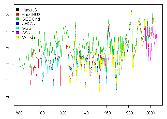
ts.plot(combine[,1:7],col=1:7)#,lwd=c(2,2,1,1,1,1,1),xlab="",ylab="")
legend(1875,2.6,fill=1:7,legend=c("Hadcru3","HadCRU2","GISS Grid","GHCN2","GISS","GSN","Meteo.ru"))
This yields this following spaghetti graph on my machine:
Now you’ll have to have installed the ncdf package and to have downloaded three large zipped files. I’ve not tried to include the unzipping of these large files in the programming since it’s probably a get idea to do this manually to be sure that you get it right. The three large files are:
HadCRUT3 – downloaded and unzipped from http://hadobs.metoffice.com/hadcrut3/data/HadCRUT3.nc into “d:/climate/data/jones/hadcrut3/HadCRUT3.nc” #5×5 monthly gridded from CRU
GISS Gridded – downloaded and unzipped from ftp://data.giss.nasa.gov/pub/gistemp/netcdf/calannual-1880-2005.nc into “d:/climate/data/jones/giss/calannual-1880-2005.nc” #2×2 degree annual gridded from GISS
GHCN Station data – # http://www1.ncdc.noaa.gov/pub/data/ghcn/v2/v2.mean.Z #unzipped, read and re-collated into “d:/climate/data/jones/ghcn/v2d.tab” #see this script for the re-collation to the R-object
HadCRUT2 – downloaded from HAdCRU and re-collated into “d:/climate/data/jones/hadcrut2/hadcruv.tab” – I posted up a script to do this some time ago, but this probably needs to be reviewed.
There may very well be some residual references to things on my computer that will need to be ironed out to make the routines fully objective. Let me know if you run into problems.
In the mean-time, you should be able to get useful components working and I hope that this helps people to wade through the gridcell data.


7 Comments
Thanks, Steve!
If someone is interested, there is a Scandinavian (up to 2002) data collection available here:
http://www.smhi.se/hfa_coord/nordklim/
A collection of excellent Denmark/Greenland data sets is available from
http://www.dmi.dk/dmi/index/viden/dmi-publikationer/tekniskerapporter.htm
Thank you very much, Steve!
I certainly don’t have your R-skills… so I’m still fiddling with the re-collated data part (GHCN Station + HadCRUT2 *.tab).
The rest however is a very straightforward thing to manage … Good work!
Downloaded the data from files found at ftp://data.giss.nasa.gov/pub/gistemp/bin/
I assume the data is the same Giss data as that which Steve linked to, just saved
in binary format.
I converted the binary yearly Fortran files into individual monthly text files.
Each file contains 3 columns. Latitude, longitude, and anomaly.
All data was 2×2 degree cell size. 16200 total cells.
From the 1880-2004 Ts files(surface air temperature). 1500 months of data.
1674 cells have one month or less with data. The next lowest count is 187 months.
3217 cells have data for all months. I get an anomaly from 1880-2004 of 0.046C.
From the 1950-2004 LOTI files(land ocean temperature index). 660 months of data.
78 cells have 11 months or less with data. The next lowest count is 148 months.
10885 have data for all months. I get an anomaly of 0.135C.
I calculated the anomaly by keeping a running total of monthly anomalies for each cell
that had 120 months of data. Calculated the mean for each cell. Totaled those values
and divided by the number of cells with 120 months.
If that’s not the correct way to do it, someone please speak up and clue me in.
I don’t have great statistical skills.
Can’t say I’m surprised by the color of LOTI image. The data starts during the cold part
of the 20th century. Still nothing extraordinary.
I created a couple maps of the data.
Colored coded: yellow > 0.5C. red > 0.0C. Green 0 to -0.5C. Blue LOTI 1950-2004
TS 1880-2004
Full-size 3600 pixels wide.
LOTI 1950-2004
TS 1880-2004
OK, so I got interested in decoding the binary data sets at ftp://data.giss.nasa.gov/pub/gistemp/download/ as well. Wrote some Perl to slice and dice the data set into various series. I now have fully 1.6Gb less free hard drive space and I cannot figure out where my Sunday went 🙂
I’ll tidy up the various scripts and post on my web site when I get a chance. The result of my attempt at visualizing TSurf1200 and SSTHadR2 combined is available on Google Video.
Enjoy.
Sinan
Josiah Charles Stamp — first director of the Bank of England and chairman of the London, Midland and Scottish Railway.
The government are very keen on amassing statistics. They collect them, add them, raise them to the nth power, take the cube root and prepare wonderful diagrams. But you must never forget that every one of these figures comes in the first instance from the village watchman, who just puts down what he damn pleases. (quoting an anonymous English judge.)
Wikipedia
This reminds of another comment by Keynes on Tingergen’s multiple correlations:
Keynes and Yule were coauthors in around 1910.
I’ve posted up Keynes comment
I took the 2×2 gridded surface temperature files for the years 1880-2004 and put them in a bar chart by latitude.
I did it two different ways. In one I simply totaled up all the data over the years by latitude and divided by the latitude data count to arrive at a mean value. That way no individual data point gets any more weight than any other.
The other way I took the mean for each year by latitude, totaled them and divided by the number of years of data for that latitude. That way each year gets the same weight. I’ve posted links to the charts below.
Point of interest. 62% of the data points are in the last 1/2 of the record.
To not bias your perspective, I suggest you decide which way you think would be a more appropriate rendering of the data before looking at it.
Using total mean. link
Using yearly mean. link