Climate Audit

If someone felt that it was necessary to detrend the bristlecone pine-based PC1 of Mann’s AD1000 network for CO2 fertilization, it’s doubtful that the initial instinct would be to coerce the data to a network of northern Canadian-Alaskan tree ring chronologies where the possibility of regional differences must surely be allowed for.

Inspection of Mann’s former FTP archive at the University of Virginia (which I fortunately archived before it was deleted) contains an interesting program entitled co2detrend.f (Mann’s main programs were not on the archive, but some programs were inadvertently left in the archive, including the program that calculated the tree ring network principal components – which was how we discovered Mann’s erroneous PC method.)

The program (which I’ve posted here) include the following interesting comments (in which Mann reports a correlation of 0.9 between the AD1000 PC1 and CO2:

c regress out co2-correlated trend (r=0.9 w/ co2)
c after 1800 from pc1 of ITRDB data

c remove co2-correlated portion (r=0.9) of 1800-1980
c
corr= 0.9

The program itself is in Fortran, which is highly verbose for simple operations like calculating a mean or standard deviation, that’s for sure. Below I’ve shown what is more or less a transliteration of his program into R so that you can see what the calculation does in simpler terms.

He first reads in the AD1000 Mannomatic PC1 and CO2 levels (with the 1610-1995 mean subtracted). I’ve uploaded both the source files to CA so that the commands below are fully operational (up to the need to take care with what WordPress does to quotation marks.) (The short R-script is here in ASCII form.)

First read in the data and make them into time series:

ser26= read.table(“http://data.climateaudit.org/data/mbh99/COMPARE/pc01.out”) # mannomatic pc1 1000-1980
ser26=ts(ser26[,2:ncol(ser26)],start=ser26[1,1])
ser12= read.table(“http://data.climateaudit.org/data/mbh99/COMPARE/ghg-lowf.dat”) # CO2 values less 1610-1995 average
ser12=ts(ser12[,2],start=1610) #this is the starting date based on other info

Then standardize the two series on the period 1800-1980 (as in the Mann program). inverting the PC1:

pc1= -ser26; #invert orienation
m1=mean(pc1[(1800:1980)-999]);sd1=sd(pc1[(1800:1980)-999]); c(m1,sd1) #[1] -0.01463 0.01858
standard1= (pc1-m1)/sd1 #1000 1980

m2=mean(co2[(1800:1980)-1609]);sd2=sd(co2[(1800:1980)-1609]); c(m2,sd2) #[1] 7.219 14.059
standard2= (co2-m2)/sd2 #1610 1980

Then subtract the CO2-adjustment from the Mannomatic PC1. The code in Mann’s program is (asum1 is the mean):

newpc1(i)=sd1*(standard1(i)-corr*standard2(i))+asum1

I implemented this as:

newpc=pc1; corr=.9
newpc[(1610:1980)-999]=sd1*( standard1[(1610:1980)-999]- corr*standard2) + m1

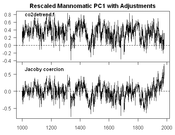
For the portion before 1610, I used the average CO2 value for the period 1610-1980 in the adjustment. Then plot. Here I’ve plotted the output from the co2detrend.f program against the “fixed” PC1 (which ties in to MBH99 Figure 1), both rescaled to match the scale of MBH99 Figure 1a.