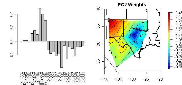
As I observed a couple of posts ago, the Stahle SWM network can be arranged so that its correlation matrix is closely approximated by a Toeplitz matrix i.e. there is a “natural” linear order. I also noted that results from matrix algebra proving that, under relevant conditions, all the coefficients in the PC1 were of the same sign; there was one sign change for the coefficients in the PC2, two in the PC3 and so on. These resulted in contour maps for the eigenvector coefficients with very distinct geometries – here’s an example of the PC2 in the SWM network showing the strong N-S gradient in this PC.

As soon as one plots the site locations and contours the eigenvector coefficients, the raggedness of the original site geometry is demonstrated. But how much does this raggedness matter? This leads us away from matrix algebra into more complicated mathematics, as the eigenvectors which contour out to the pretty gradients in the earlier diagrams now become eigenfunctions with an integral operator replacing the simpler matrix multiplication.
As an exercise, I thought that it would be interesting to see what happened in an idealized situation in which the network was a line segment with spatial autocorrelation as a negative exponential function of distance between sites.
Because all the circumstances are pretty simple, one presumes that the resulting functions are simple and I presume that there’s a simple derivation somewhere for eigenfunctions in these simple cases.
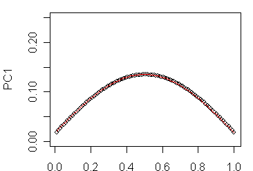
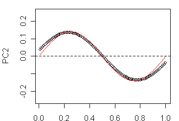
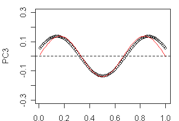
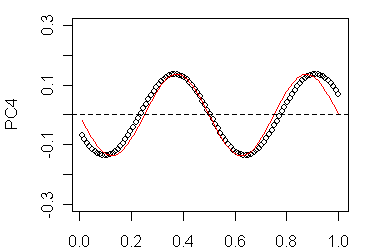
Since I don’t know these derivations, I went back to more or less brute force methods and did some calculations using N=51; N=101,… , assuming that the sites were uniformly spaced along the line segment, creating a correlation matrix for rho=0.8, carried out SVD on the constructed correlation matrix, plotted the eigenvectors and experimented with fitting elementary functions to the resulting eigenvectors. As shown below, I got excellent fits (with some edge effect) for the following eigenfunctions:
where k = 1,.. and t is over [0,1].
So it looks like the eigenfunctions are pretty simple. One can also see how the number of sign changes increases by 1 as k increases by 1.
 |
 |
 |
 |
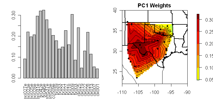
Even the plots in the network illustrated yesterday show elements of these idealizations. For example, here’s the PC1 from the combined network. I think that I can persuade myself that there are elements of the sin (kt) k=1 shape from the idealized PC1 coefficient curve illustrated in the top right panel.
Next here’s the PC2 from the combined network. Again I think that I can persuade myself that there are elements of the sin (kt) k=2 shape in this example.
Obviously the functions are elementary and I’m sure that there are any number of elegant derivations of the formulas. But I think that the results are at least a little bit pretty in the context of something as humdrum as the Stahle SWM network. As one goes from a 1-D to a 2-D situation, the geometry is somewhat more complicated, but we’re still going to see well-constrained relatively elementary functions making up the eigenfunctions for squarish and rectangular shaped regions.
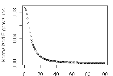
Also, here’s a plot of the normalized eigenvalues for N=101. Again, I’m sure that there’s a known distribution for these eigenvalues somewhere in the mathematical literature and would welcome any references.


12 Comments
My first guess would be that Hermite-Gaussians would be a typical basis for your eigenfunctions. They come up all the time in rectangular problems. See for instance gas laser transverse modes. If it were properly cicular geometry you’d use Lebesgue-Gaussians. But this is just a feeling.
Try this:
Click to access Spectra_Physical%20Rev%20E%2063,%20026704%20(2001).pdf
Steve: It’s about eigenvalues, but for circumstances quite different than the ones at hand and do not derive results that are on point for the present situation.
It looks like the PC transform has useful similarities with Fourier or Laplace transforms. Could you borrow some knowledge from these well-studied transforms?
#3. This is a very specialized case. Quite different sort of results occur when you get inhomogeneous systems.
Click to access North-Sampling-1982.pdf
You lost me at “eigenvector coefficients”. Can anyone translate this entry into English for us common folk?
English: Some of the crucial bits of the current “best temperature reconstruction” are essentially the mathematical equivalent of zero divided by zero. Not only did they start with problematic data (tree-rings are precipitation sensitive), but then they used a method that unduly weights individual sets of data by their geographic relation to other points. Four points in a perfect square would be equally weighted. But if there were three in an equilateral triangle with one dead center, the dead center data point is going to basically be counted twice. It is more complex with non-geometric figures.
This highlights and exacerbates something that is known as ‘cherry picking’. The “best temperature reconstruction” doesn’t use all tree-ring studies. Or all tree-ring studies that were actually taken with temperature-tree-ring studies in mind. Instead, they were chosen on how well they “worked”. And some of the non-included data was then not archived on the basis “Well, I didn’t use it.”
So you can have a lone hockeystick treering and emphasize that particular signal with completely flat treering signals by just making sure that the flat ones are spaced around the periphery and the ‘key’ treering is centrally located. I’d actually like to see this simplified scenario carried out, just to emphasize how much the choice can be affecting things.
Thanks Al. That’s much better.
#7 is not a translation of the post, but raises different matters. I can’t translate everything into simpler terms; this is already a more plentifully illustrated exposition of the point than you’ll find anywhere. If you don’t get all the nuances, don’t worry about it.
I get the entire engien thing as operators on vectors.
Vectors are arrows if you will. A geometric magnitude and direction. Collections of these form vector spaces which can be scaled and added. Linear transformations can be made on vectors. So if I take a vector and double its length but not the direction, the eigenvector has an eigenvalue of +2 If I reverse the vector and double its length, I have an eigenvalue of -2
So eigenvectors are the already transformed lines which are described as being different from the original by looking at the eigenvalue.
Then you start getting into different ways you can change each vector in a vector space and combinations, and then you get into math using matrices. And that’s where I stop.
These mgiht help.
http://members.aol.com/jeff570/e.html
http://planetmath.org/?op=getobj&from=objects&id=4397
Or this online linear algebra lecture #21 (so it might require some prerequite knowledge…) 😀 :
http://video.google.com/videoplay?docid=-8791056722738431468&hl=en
And a calculator
http://www.arndt-bruenner.de/mathe/scripts/engl_eigenwert.htm
Hi, I am trully late for this party.
I am not sure whether this is the best place to post this as it also refers to a later posting but here will have to do. I am reasonably sure of the following but it is not well grounded in any literature of which I am aware.
In the later post a link to Chladni Patterns is drawn which I think might possibly mislead. The vibrational patterns on a disc are determined by real boundary conditions, for the plate has real edges.
The similar patterns that appear in autocorrelated data may be determined simply by the subjective choice of the observational area, window or aperture. I guess this is your point.
The same is true of an autocorrelated causal time series. The eigenvectors for a specified autocovariance and segment length are always the same relative to the segment being analysed. Move the segment or aperture to an earlier or later time whilst preserving its length N, and the eigenvectors move with the aperture. They are not an any normal sense real.
I say this as there might be a temptation to encourage our thinking that the real data elements in the middle of an aperture necessarily behave differently to those at the extremities. If you sum the total variance for any data element according to the eigenvector/eigenvalue pairs you will get the same value but it will be distributed across the eigenvector/eigenvalue pairs differently. However a problem arises if you decide to discard any of the low order eigenvectors, the ones with small eigenvalues as you are forcing a pattern on the now filtered data that would tend to move if you moved the aperture.
The eigenvectors across an aperture in a time series are also either symmetric and antisymmeric despite the asymmetry of the autocorrelation function for all causal functions.
Having said that the eigenvectors may be determined by observer choices, that is not to say that they are arbitrary to the analysis. They have the property that upto any possibly degeneracy they form a unique basis for which the eigenvalues are all fully independent. I believe all other choices for an orthogonal basis will have weighting values drawn from distributions that are correlated. Also filtering by removing the variance attributable to any vector other than an eigenvector will leave a residue that when projected back on the existing eigenvectors or perhaps those resulting from the analysis of the filtered system, (which will have one less degree of freedom), will result in weights and eigenvalues that are correlated. Typically neither the mean nor a linear slope are eigenvectors and similarly their removal results in a residual that is not fully independent of the values of the mean and gradient removed, this is normally very minor but worth mentioning given statistical tests tend to assume that the residuals are fully independent of the variance of the vectors removed.
As the eigenvalues act like fully independent random variables, each adds seperately to the total expected variance. As each eigenvector/eigenvalue pair has a different expected variance, the total variance may have a distribution similar too, but definitely not Chi-squared even for normally distributed generating noise, this divergence from Chi-squaredness has I think the potential to cause problems but probably less so than the difficulty in constraining model paramaters to a small enough region to avoid a Bayesian analysis under uncertainty in the parameters.
The eigenvectors represent a basis where the expected variance attributable is maximised for each eigenvector in turn. That is the expected variance as approximated by PCA/EOF type analysis over a large number of independent samples. That is to say if one analysed the mean temperatures for each day in August this year its representation according to the eigenvectors of the 31 day aperture with its known or suspected autocovariance function would not be very revealing but a compilation of many different years of August values would reveal the eigenfunctions. Move the aperture to say, mid-July to mid-August and the sample weights would change, yet for a large sample, the sample EOFs would largely stay the same relative to the aperture, not to the data unless some real effect existed; the underyling eigenvectors as determined by the aperture size and the autocorrelation would stay the same relative to the aperture.
With regard to time series, there is another group of eigenvector/eigenvalue pairs of interest, those that represent the effect of events prior to the start of the aperture chosen for observation or analysis, on the data in that aperture. I will call them the history eigenvectors if you will allow.
Famously AR(1) has a single history eigenvector, an exponential decay. ARMA(1,1) also has a single history eigenvector and in general ARMA(p,q) has the greater of p and q eigenvectors provided that is no greater than the aperture length N. So for most ARMA(p,q) functions the historic content of the data in the aperture will not have a large number of degrees of freedom as compared to models that have longterm persistence where the historic DOFs may only be limited by the length of the aperture. The historic eigenvectors are of course anything but symmetric across the aperture, typically they each have an initial offset and a trend that reverts to the mean perhaps with damped oscillations. I believe that these will also suffer correlation in the expectation of the eigenvalues whenever the mean, as is almost universally the case, and or the gradient have been filtered out. That is to suggest that to simulate possible history functions for observed data one might prefer to simulate the full history eigenvectors using suitable noise weighted by their eigenvalues and then filter out the mean and gradient as applicable. To make this clearer, to simulate ARMA(5,3) data one could calculate the 5 historic eigenvector/eigenvalue pairs for the following aperture drive these by 5 of the random noise variables and combine this with an aperture driven assuming all the prior noise variables were zero, which can save using the very long run in necessary models other than AR(1), and also facilitate querying what plausible prior history could have contributed to the observed data.
In a similar but not identical way the expected observational lagged covariance or correlation function must be determined for the particular aperture size whenever, as is generally the case, the mean and possibly the gradient has been removed. Loss of the mean gives rise to the typical tendency for the now filtered sample covariance/correlation function to cross through to negative values for some lag even when the full covariance function doesn’t. Again the observed sample covariance function can be decomposed into its expected part which has a weight representing a variance which for normal generating noise has a pseudo Chi-Squared distribution in much the same way as above, plus I suspect some eigenvectors whose eigenvalues represents a product-normal distribution but I am unsure of the details. The point here being that the expected part of the lagged covariance functiion for any arbitrary response function is computable according to the aperture size but even so the observed covariance/correlation function is but one instance of the sum of the expected part with some unknown weight plus all the nuisance parts and determining unique model parameters from a single observation is fraught in the well known way that it is. However it may be possible to see when the model is inadequate in cases where particularly the long lagged covariance is much larger than plausible for models that lack true longterm persistance, this seems to me to be the case for typical sample temperature series, ARMA(p,q) models are commonly quite well constrained at the long lag extremity of their covariance function.
To summarise, I believe that EOFs/PCAs may commonly be largely a function of the observing aperture but not necessarily so, and that this may not be obviously the case in particular circumstances. Any procedure akin to EOF/PCA analysis will tend to converge to the underlying eigenvectors whenever there is no real feature present in the data and in that case moving the aperture will move also move the EOFs/PCAs largely unchanged but will alter their weights. I think that the potentially phantasmagoric nature of all this is covered in the posts that follow.
Alex
I appreciate the comment. The Chladni posts are among my favorites in the entire CA corpus and I welcome any thoughts on the topic, especially well-considered ones like this.
I am convinced that Chaldni patterns recur in some borehole inversions as well, though I only have notes on the topic.