One of the longstanding CA criticisms of paleoclimate articles is that scientists with little-to-negligible statistical expertise too frequently use ad hoc and homemade methods in important applied articles, rather than proving their methodology in applied statistical literature using examples other than the one that they’re trying to prove.
Marcott’s uncertainty calculation is merely the most recent example. Although Marcott et al spend considerable time and energy on their calculation of uncertainties, I was unable to locate a single relevant statistical reference either in the article or the SI (nor indeed a statistical reference of any kind.) They purported to estimate uncertainty through simulations, but simulations in the absence of a theoretical framework can easily fail to simulate essential elements of uncertainty. For example, Marcott et al state of their simulations: “Added noise was not autocorrelated either temporally or spatially.” Well, one thing we know about residuals in proxy data is that they are highly autocorrelated both temporally and spatially.
Roman’s post drew attention to one such neglected aspect.
Very early in discussion of Marcott, several readers questioned how Marcott “uncertainty” in the mid-Holocene could possibly be lower than uncertainty in recent centuries. In my opinion, the readers are 1000% correct in questioning this supposed conclusion. It is the sort of question that peer reviewers ought to have asked. The effect is shown below (here uncertainties are shown for the Grid5x5 GLB reconstruction) – notice the mid-Holocene dimple of low uncertainty. How on earth could an uncertainty “dimple” arise in the mid-Holocene?
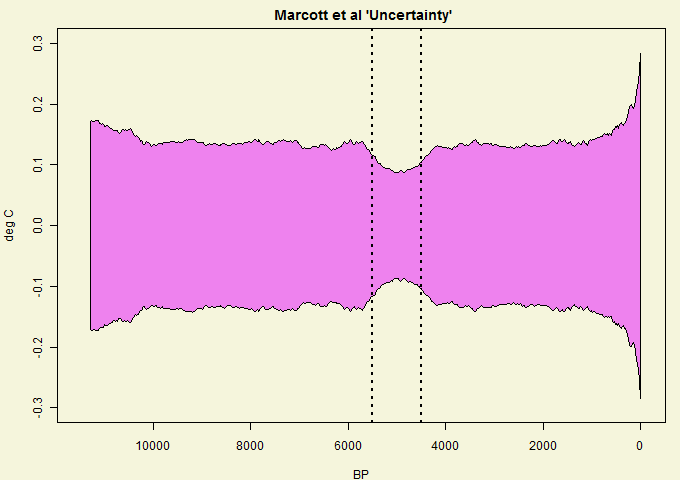
Figure 1. “Uncertainty” from Marcott et al 2013 spreadsheet sheet 2. Their Figure 1 plot results with “1 sigma uncertainty”.
It seems certain to me that “uncertainty” dimple is an artifact of their centering methodology, rather than of the data.
Marcott et al began their algorithm by centering all series between BP4500 and BP5500 – these boundaries are shown as dotted lines in the above graphic. The dimple of low “uncertainty” corresponds exactly to the centering period. It has no relationship to the data.
Arbitrary re-centering and re-scaling is embedded so deeply in paleoclimate that none of the practitioners even seem to notice that it is a statistical procedure with inherent estimation issues. In real statistics, much attention is paid to taking means and estimating standard deviation. The difference between modern (in some sense) and mid-Holocene mean values for individual proxies seems to me to be perhaps the most critical information for estimating the difference between modern and mid-Holocene temperatures, but, in effect, Marcott et al threw out this information by centering all data on the mid-Holocene.
Having thrown out this information, they then have to link their weighted average series to modern temperatures. They did this by a second re-centering, this time adjusting the mean of their reconstruction over 500-1450 to the mean of one of the Mann variations over 500-1450. (There are a number of potential choices for this re-centering, not all of which yield the same rhetorical impression, as Jean S has already observed.) That the level of the Marcott reconstruction should match the level of the Mann reconstruction over 500-1450 proves nothing: they match by construction.
The graphic shown above – by itself – shows that something is “wrong” in their estimation of uncertainty – as CA readers had surmised almost immediately. People like Marcott are far too quick to presume that “proxies” are a signal plus simple noise. But that’s not what one actually encounters: the difficulty in the field is that proxies all too often give inconsistent information. Assessing realistic uncertainties in the presence of inconsistent information is a very non-trivial statistical problem – one that Marcott et al, having taken a wrong turn somewhere, did not even begin to deal with.
I’m a bit tired of ad hoc and homemade methodologies being advanced by non-specialists in important journals without being established in applied statistical journals. We’ve seen this with the Mannian corpus. Marcott et al make matters worse by failing to publish the code for their novel methodology so that interested readers can quickly and efficiently see what they did, rather than try to guess at what they did.
While assembling Holocene proxies on a consistent basis seems a useful bit of clerical work, I see no purpose in publishing an uncertainty methodology that contains such an obvious bogus artifact as the mid-Holocene dimple shown above.


198 Comments
Typo here? “centering all series between BP4500 and BP500”
Should be BP5500 perhaps, to match the figure?
Marcott et al. would bark with defiance
At suggestions they place high reliance
On these artifacts…
Of course, if it lacks
Such weirdness, it’s not “Climate Science”!
===|==============/ Keith DeHavelle
All true, but… if you want to see real statistical illiteracy in action take a look at the medical research published by doctors working and teaching at even our most revered universities (and yes, including the top two).
Academic research publishing on most subjects really consists of just bricks being used to build careers. It’s only when relatively rare attempts are made to use the product in the real world and measure the result that it becomes important whether the conclusions are reliable. When outsiders make a fuss about this academics make efforts to shape up, but as you point out the results are usually laughable.
To see how intractable the problem is, try suggesting that a working research academic take a statistics course just one level up from wherever their (often minimal) understanding is now.
Steve:
I believe the visual equivalent of your dimple can be seen at Nick Stokes’ visual summary of the proxies. Is this visual dimple “real” or artifact?
In addition, if you have a bunch of proxies with very small relative change in anomalies over an extended period of time then wouldn’t you get a dimple? But then how meaningful or useful is the series as a temperature proxy?
Steve: the dimple comes from the centering on the mid-Holocene, not from the small changes per se.
Bernie,
You’re right, and I’ll give a technical answer which relates to the dimple. Each curve there has the 4500:5500 mean subtracted. That is, they are shifted to minimise the sum of squares deviation (even total SS for all curves) in the range. That’s what you’re seeing. For another range, say, 2500:3500, the thing subtracted does not minimise the SSD. It’s much larger.
Nick:
If that is so then what uncertainty is Marcott et al actually measuring?
In addition, my understanding is that anomalies are valuable to identify trends. Here anomalies seem to be being used for something else – more akin to z scores or some kind of normalized score. But with z-scores you would use the entire set of data for each proxy.
Bernie,
I said below that Marcott is measuring exactly what Craig Loehle measured, and in the same way (with applause from CA). And what everyone else does. If you have a disparate proxy set, you have to put them on the same basis. Otherwise you can’t proceed.
You do that by subtracting from each one some reference value – usually a mean over some period. That makes it an anomaly. Then you take some kind of mean of the anomalies. That makes it a recon. It’s not a recon of some absolute temperature – that just can’t make sense. It’s a recon of an average anomaly. And the CIs are those of that average.
I can’t think why that would be the best way to deal with a disparate proxy set. The number of implicit assumptions in that particular method seems to throw away a lot of info.
“It seems certain to me that “uncertainty” dimple is an artifact of their centering methodology, rather than of the data.”
Well, it’s a consequence of the definition of what they are plotting – the uncertainty of anomalies defined relative to the 4500-5500 base. If they had defined the anomaly relative to the actual or interpolated value at 5000BP, as they could, they would, correctly, get zero uncertainty there. The anomaly there is guaranteed to be zero.
Steve: Nick, you’re Racehorse-Haynesing again. Their captions refer to anomalies 1961-90. Further, if their definitions lead them to a nonsensical result – as here – then they should redo their analyses.
“Their captions refer to anomalies 1961-90.”
The individual proxies are set to a base period of 4500-5500BP. That’s when the CIs are determined. The aggregate recon subsequently has an offset added to bring it in line with 1961-1990 via CRU/EIV. That doesn’t change the uncertainty intervals.
The “nonsensical result” is not a result of the analysis. It’s a result of the anomaly definition. There really is a dip in uncertainty of the anomaly. It’s absolutely necessary to deal with anomalies – there’s no other way to aggregate icecores, tropical deep sea etc. A broader base period would have slightly reduced the effect. But too broad, and some proxies would have missing segments.
Re: Nick Stokes (Apr 7 16:13),
Nick,
do you agree that the supposed mid-Holocene minimum in “uncertainty” is an artifact of the marcott methodology? Or is it your position that, as Ross puts it, there was a real Mid-Holocene Stochastic Attenuation?
I obviously do not believe that there was a Mid-Holocene Stochastic Attenuation and therefore believe that marcott et al have left something out of their calculation of “uncertainty”.
Because you and Marcott have defined “uncertainty” in a stupid way doesn’t mean that your definition has any meaning or should be accepted. Indeed, as I observed in the post, one of the major problems in this field is that people holding themselves out as qualified to conduct statistical analysis of complicated data sets have no training and less aptitude and come across as the statistical equivalent of skydragons – a category in which you too often locate yourself.
“I obviously do not believe that there was a Mid-Holocene Stochastic Attenuation and therefore believe that marcott et al have left something out of their calculation of “uncertainty”.”
No, there is nothing left out. It is simply a consequence of the definition of what it is they are expressing the uncertainty of.
If you look at their calculation method, SM sec 3, in step 4, after perturbing each individual record, they subtract the mean from 4500-5500. That is what anomaly means. For each age point, this is done for each of the 73000 proxy/MC datapoints.
Then they calculate the mean and sd of those 73000. The sd generates the uncertainty.
As I said above, if their definition had been “anomaly relative to 5000BP”, then all 73000 values would have been zero, by definition. The mean and sd would have been zero.
As it is, the sd is reduced in the range. Suppose an individual age seq had a positive blip in the 4500-5500range. That would normally increase the uncertainty estimate there. But it pushes down the mean of that age seq (one of the 73000), which is subtracted from that seq, reducing the effect of the uncertainty. A similar excursion outside the range would not trigger that compensating effect. Hence the dip. This is not some Marcott special; it is simply the correct way of implementing anomaly.
To choose to calculate an anomaly with a specified time range is not controversial, and there is little alternative. The rest follows.
Multi-variables can be confusing, so I’d better expand a couple of phrases above:
“For each age point, this is done for each of the 73000 proxy/MC datapoints.”
Marcott’s cube is age (565) x dataset (73) x MC (1000)
For each of the 73*1000 age sequences, the 4500:5500 average for that sequence is subtracted from that sequence.
“all 73000 values would have been zero, by definition”
If the range had been 5000:5000 then every one of the 73000 sequences would have age=5000 equal to zero.
Ah but this is climate statistics, not regular statistics.
Just like multivariate regression methods have the advantage of being insensitive to the sign of predictors, anomaly methods have the advantage of reducing the uncertainty in particular regions of the reconstruction.
That this is physically absurd is neither here nor there, and to consider the physical meaning of the results is just bizarre.
🙂
Am I doing it right?
Spence_UK (Apr 8 02:17),
I think their horrible method is more akin to Mann’s “off-centered” PCA. There is no reason nor need to center the proxies on any other interval but the full.
Jean S,
“I think their horrible method is more akin to Mann’s “off-centered” PCA. There is no reason nor need to center the proxies on any other interval but the full.”
It is what is done by all the surface temperature indices (1961-90 etc). But with full centering, how would you deal with proxies that don’t span the interval?
Jean S, I agree that mathematically it is more like the short centring issue. People forget that the anomaly method – whilst important for climate analysis – injects errors into the analysis, and it is important to understand, minimise and account for those errors.
But in terms of the excuse wheeled out by Nick (that a characteristic of the methods employed should be more important than physical meaning), this reminded me very much of Mann’s PNAS response. I couldn’t resist connecting those dots.
Nick Stokes (Apr 8 06:30),
Which is pretty funny comment considering that Steve started by saying:
A simple (but still better) thing to do is to use the full overlap. There are better ways of handling this, but IMO it is a waste of time to try to discuss anything of substance with you. If you truly are interested in the issue, start by reading Little&Rubin: “Statistical Analysis with Missing Data”.
Jean S,
Surface temperature indices are not paleoclimate, and organisations like NOAA do not lack access to statistical expertise. The indices have been used and quoted extensively at CA; no-one has to my knowledge said their use of fixed anomaly period it is a horrible method akin to PCA.
I’m sorry that you can’t help with the very substantial problem that prevents people using full overlap.
Nick Stokes (Apr 8 08:00),
Oh, really. And I was under the impression that one of the main points of the reference station method (Hansen & Lebedeff), the first difference method (NOAA), and now the new BEST method was the avoidance of a “fixed anomaly period”. But everyone has their own statistical authorities, and in your case it seems to be Excel-challenged Jones. And now I get back to my usual and intended mode of ignoring you.
Jean S,
“And I was under the impression that one of the main points of the reference station method (Hansen & Lebedeff), the first difference method (NOAA), and now the new BEST method was the avoidance of a “fixed anomaly period”. “
You were misinformed. Hansen and Lebedeff used a fixed anomaly period (1951-80). GISS still does. NOAA used a fixed anomaly period (1961-90). They now use sometimes 1981-2010, sometimes 1901-2000. BEST is different.
The purpose of the reference station method, and the first difference method is to allow anomaly calculation where data is missing during the fixed period. Such precautions are essential, to avoid introducing spurious trends. They would be required in any paleo calculation with proxies that do not have data in the full period. But I have not seen it done. That’s why I wondered what you had in mind.
If all stations have sufficient data in the anomaly period, RSM and FSM are redundant.
Nick – can you think of (and share) any physical basis that would explain their pattern of uncertainty?
This brings to mind and old song:
“She’s got dimpled cheeks.
I never cared for dimpled cheeks
But she’s got dimpled cheeks
And that’s my weakness now.”
Nick’s just in love.
Again, uncertainty of what? When you’ve answered that properly and in full, it’s clear.
Nick, I’m going to bring over a comment you made in the Quelccaya thread: “I’m not aware of any multiproxy jockeys using a single site as proxy for world temperature”. I would agree with the idea that measurements of a single site are not global measurements. Putting aside the dimple, here’s my question to you (or anyone else), since multiproxy studies are not multiple measurements of a single phenomena, does it even make sense to use standard deviation as a measure of uncertainty?
As a simple example, if I want to find the mean height of everyone in my family, I would measure everyone and take the mean. My confidence in that value would not be defined by the SD of the heights, but would be based on the confidence of the individual measures.
mt,
“does it even make sense to use standard deviation as a measure of uncertainty?”
You have to manage with what measure you can get. But to look at your family example, the thing is that you’re not thinking of your family (height distribution) as part of a larger population. So all you need to worry about is error in the mean arithmetic.
But we aren’t interested in the actual mean of a whole lot of icy and wet places. We’re looking for these measures to tell us something about the whole Earth. That is what the mean is meant to represent.
So the question is, what if we did similar experiments with maybe different proxies. Or even different bits of the same cores. How much is that recon (mean) likely to fluctuate.
That’s why the variation between proxy anomalies is important. It’s obviously not an ideal measure because of their heterogeneity, spatial sparsity etc. And they possibly could have supplemented it with a study of variation of each proxy over time. But it’s the measure that we have.
Re: Nick Stokes (Apr 8 20:38),
And if our result is physically nonsense… do we accept it as is and call it good, or recognize that a mistake is being made?
There’s such a thing as floor to ceiling CI. Sometimes, that’s the actual result. Frustrating yes. Don’t hide it… if we do, then we’re only fooling ourselves. Very unscientific.
Re: Nick Stokes (Apr 8 20:38),
Said with a smile: a dead horse doesn’t move much either. But it has a rather limited ability to tell me much.
Just because we get a bunch of nice looking data does NOT mean we have learned anything.
There are endless posts here at CA about this.
‘night
Nick, thanks for the response. I can understand using mean as a crude approximation of a reconstruction, but it doesn’t necessarily follow that standard deviation would be a reasonable measure of uncertainty. To put my question a different way, does using standard deviation for uncertainty mean there’s an implicit assumption that the individual proxies are measuring global temperature?
Second, “But it’s the measure that we have.” Assuming you’re talking about SD here, no, it’s the measure that Marcott et al used. It seems to me there are at least three individual sources of uncertainty, the measurements themselves, sparse sampling, and the method of reconstruction. I don’t think the SD across the proxy series is any of those. In fact, variation across proxies for a given time point should be expected (see globe vs Peru vs southern Peru vs Quelccaya proxy for the ’98 El Nino)
Re: Nick Stokes (Apr 7 13:51),
That’s an interesting claim, Nick. Seems true on the surface, yet I quickly begin to wonder.
I think you are saying this; please tell me if I am wrong:
1) We have a base series B and a proxy series P.
2) Anomalies are calculated (horribly oversimplified: A = P-B) relative to a particular date or date range in the base.
3) If the baseline reference were a single point in time, then by definition the anomaly uncertainty at that point in time will be zero.
I can’t stop anyone from reading further right away, but I would ask you to consider the above carefully before continuing.
My observation:
It is true that the anomaly could be calculated to be exactly zero at the exact point in time of calibration.
Yet… why in the world should that imply that the uncertainty of the anomaly ought to be zero at that point? Seems to me the calculation method, and the calibration point or range, should have exactly zero influence on the uncertainty.
Isn’t “zero” an arbitrary value in this situation? Thought experiment: calculate offset anomalies where the “zero point” is 1 degree offset. Should that have any impact at all on the uncertainty/CI? I think not.
MrPete,
I think I’ve covered this in my answer to Steve above.
To continue the measuring height analogy, if I change all the measurements to anomalies based on one person’s height, that doesn’t mean there is no uncertainty in the anomaly of the “standard” person’s height. There is still uncertainty based on the fact that my original measurement of the standard wasn’t certain.
Which gives me the minimal opening I wanted to thank both you and Steve McIntyre. I’m never sure I’ve understood one of these statistical issues well enough to have an opinion, one way or the other, until both of you have spoken on it.
What puzzles me, is that they don’t seek advice before applying their home made methods. As a young student who had taken a couple of statistics courses, I assisted a biology professor with a biostatistics project (which wasn’t too different from paleoclimatology, some of it involved correlations between microorganism shapes and ecological factors). I consulted a statistics professor to make sure we didn’t draw the wrong conclusions from our stepwise regression runs, and when I reinvented (n-means) cluster analysis, we took the analysis to a botany professor with more experience in biometric methods who could tell me what I had reinvented 🙂
Something tells me there might be a cultural thing in medicine and climate science, a case of hubris, that makes this behavior more common than in other branches of science. Or at least I hope so, for the sake of science in general.
It’s simpler than that. It means adding an extra name to the author list with an implied admission of some gap in your own knowledge and a dilution of ones own role.
In defence of home brews it is often possible to match the answer more precisely to the question asked if you concoct your own statistic. By confining yourself to textbook procedures (for example to be able to apply existing tabulated significance levels) it is commonly necessary to reframe the question and then it no longer matches the “reality” one is trying to model.
Of course it is then incumbent on you to develop the significance tables or the sampling properties of the home brew procedure which in these days of computer simulation is not necessarily a big deal.
When using home brew methodoligy there is always the risk of bending your methods around to make the data produce the results that you want to see. Not nesesarily fraud. Its just that you become so desprate to prove your belief that you might overlook things. It can be hard to take, if your homebrew method proves you wrong.
thing Blondot and his N-rays 1903.
http://en.wikipedia.org/wiki/N_ray
without being established in applied statistical journals.
=================
In what other field of science is it acceptable or even recognized to “invent” your own mathematical techniques and numerical methods?
If the methodology has not already been vetted by the mathematical and statistical community how can the results be trusted in any fashion?
Should this not be a primary requirement of any scientific paper? If you are going to use a novel method to analyses the data, then first publish a paper on the method.
Only after the method has been analyzed and accepted by the mathematical and statistical community should it actually be used.
Otherwise, what is happening is that there are two different studies over 1 paper. One study is trying to analyze their statistical methods to see if their methodology is valid from a mathematical point of view.
The second study is trying to see if their conclusion match the results from a climate science point of view. Under the assumption that the statistical and numerical methods are correct.
The problem is that this leads to conflict because the two groups may reach two entirely different opinions about the validity of the paper, and each group will be arguing that they are correct.
What should be recognized up front is that unless and until the mathematical and statistical methods have been validated by the mathematical community, there is no point in analyzing the finding s as to their impact on climate science. The assumption that the math is correct may to turn out to be false.
It perhaps might be a means to minimize the potential for conflict to formalize this approach, to not contest the climate science conclusions but simply to note that they are null and void until the statistical methodology has been accepted by the mathematical and statistical community.
ferdberple, as already mentioned, medicine is such a field of science. I think I might have mentioned it on CA before, but for your entertainment: Here’s the medical researcher that reinvents integration all by himself without the help of Archimedes or Riemann and gets a boatload of citations: http://fliptomato.wordpress.com/2007/03/19/medical-researcher-discovers-integration-gets-75-citations/
In this weekend’s WSJ E O Wilson, the world’s leading expert on ants, claims that great scientists don’t need math.
“Without advanced math, how can you do serious work in the sciences? Well, I have a professional secret to share: Many of the most successful scientists in the world today are mathematically no more than semiliterate.”
http://online.wsj.com/article/SB10001424127887323611604578398943650327184.html?mod=WSJ_LifeStyle_Lifestyle_5
It seems that Climate Audit regularly proves the lie to this claim.
Steve: Hmmmm. It seems to me that Climate Audit regularly proves the opposite: that many of the world’s most “successful” climate scientists are “mathematically no more than semiliterate.” But semiliterate in the opposite way to the ant guy: the ant guy doesn’t pretend to know things that he doesn’t know. With Mann, Marcott and that crowd, they have the Mark Twain/Satchell Paige problem: it’s not the things they don’t know, it’s the things they “know” that ain’t so.
snip – overeditorializing
This post makes the fact this paper got by peer review in Science that much more astounding.
As someone who passed his Ph.D exams in econometrics, I appreciate Steve’s comments about using home brewed, unvalidated techniques. Defies common sense.
Suggest Steve should offer some excerpt to the editors of Science. Perhaps this episode can help them mend their ways, independent of the specifics of the Marcott paper, since the problem is apparently also rampant in medicine.
I can personally say it is also present in nanotechnology and energy storage. A refined method of reporting ‘truthful’ but 50% exaggerated results has even been developed by practioners like Gogotsi from the Drexel Nanotechnology Institute, which gets headlines and cover stories in Science despite being provably wrong and totally misleading.
Proofs available upon request, although different physics than climate.
Less a dimple than a wasp waist. Looks like they pulled the corset too tight.
It might be that the “mid-Holocene Climate Optimum” refers not to temperature, but to a worldwide, temporary reduction in randomness. In that case the proxies are accurately registering the event. This could even be a test of future reconstructions: do they accurately capture the Mid-Holocene Stochastic Attenuation, with its well-established teleconnections to ENSO and high elevation bristlecones?
Optimum [climate science] noun – a paleoclimatic period evidencing a defined reduction in randomness. e.g., Marcott et al. (2013).
This optimum reduction in randomness is clearly visible in Fig. Holocene Temperature Variations.png under Holocene climatic optimum as established by the postmodern standard of science, Wikipedia.
🙂
Superb Ross. We need a “like” button!
Ross is on to something. Perhaps Marcott et al is approaching an understanding of new math and emergent phenomena, which will eventually lead to the Infinite Improbability drive.
https://en.wikipedia.org/wiki/Technology_in_The_Hitchhiker%27s_Guide_to_the_Galaxy#Infinite_Improbability_Drive
In September 2013 Marcott et al 2013 is still highly praised by Stefan Rahmstorf http://www.realclimate.org/index.php/archives/2013/09/paleoclimate-the-end-of-the-holocene/
and Gavin Schmidt prefers these kind of data to adjust his climate model sensitivities http://www.realclimate.org/index.php/archives/2013/09/on-mismatches-between-models-and-observations/comment-page-1/#comment-408404
even after all the criticism written here.
@Ross McKitrick- Genius irony.
Centring is required, but difficult choices. Using the whole record would be good, but the records are different lengths. Using the modern value, would be good, but many of the records stop short of the modern period. Using instrumental data would be great, except that there might be systematic offsets between the instrumental data and the proxy. Briffa and Osborn (2006) had a methodology that coped with different length records.
But the important question is, does it the choice of centring periods materially affect their conclusions?
Steve: the issue is whether their “uncertainties” properly represent the actual uncertainties of the reconstruction given inconsistent proxies. This question is not equivalent to the choice of centering period. The graphic here shows that something is wrong with their calculation. How does one do it right? As I said, it seems non-trivial to me.
How do you determine if proxies are inconsistent? Yes, in a region, proxies should have a similar profile (or they are responding to different aspects of the environment, or are just noise). I wouldn’t expect reconstructions from the Nordic Seas and Antarctica to be consistent on sub-Milankovitch timescales.
Richard,
If you will excuse the late interruption, the question which the paleoclimate field needs to be answering is not “how to determine that proxies are inconsistent”, but rather how to determine that they are consistent. Far too much weight is given to these papers.
While it is neat to find correlation between various proxies of the same type and location, none of that means “temperature” to me and none of it proves long-term consistent response. I really want to know historic temperatures, yet find nothing in proxy reconstructions which has any solid meaning in the last 1000-10000 years.
In my opinion, the CI of this particular paper (and many other paleo papers) is a complete joke in that it doesn’t have anything to do with the confidence of knowledge of actual temperature. I have read far too many paleo papers, some even with normal rational math, to not have any confidence whatsoever in historic temps and that is disappointing.
Re: Jeff Condon (Apr 9 07:38),
Jeff, are you saying paleothermometry is a crock?
Beta,
I have never read a last 10K years paleo paper which convinced me that it was showing actual temperatures. On review of the various proxies from speleothum, boreholes, trees, there is nothing which gives me any confidence that the wiggles are at all related to temperature. With careful deconstruction, some of the best known papers are statistically NOT temperature, despite their claims.
Some people may know the field better than me and can point me to some work which would help, but I am hardly a complete rookie in this field.
What would persuade you?
For example, there are well over 100 records that show the early Holocene was warm in the northern mid-high latitudes. These results, from over a dozen proxies with different physical or biological bases, are mostly coherent regarding the magnitude and location of warming. Is that not good evidence that the early Holocene was warmer? Can we not use the temperature estimates as an indicator of the magnitude of temperature change?
Yes some of the proxies are not sensitive to the aspect of climate they are supposed to represent, and some authors are over-optimistic about the uncertainties of their proxy.
Richard, as you observe, there are a number of lines of evidence supporting high-latitude early Holocene warmth. Speaking for myself, I don’t doubt the phenomenon.
You ask: “Can we not use the temperature estimates as an indicator of the magnitude of temperature change?” If that’s what one is interested in – and it seems interesting to me, then the starting point would seem to be an analysis of the estimated differences from the various proxies.
Where matters seem to go awry is when the data gets homogenized by the multiproxy jockeys without proper care. In the case of Marcott, trying to estimate the differences by centering the proxy data in the mid-Holocene, averaging the data so centered, then recentering on the Mann et al 2008 EIV reconstruction seems a really, really bad way of trying to do this.
I agree with Jeff’s criticism of the methods employed by the multiproxy jockeys. Again, this doesn’t mean that it’s impossible to do analysis, only that the proffered analysis is not adequate, as with marcott. Even if there is some residual point in their study, it is ridiculous that a prominent study in an important journal should contain an embarrassing and obvious error on the uptick. In my opinion, it’s an error, not simply a matter of non-robustness, and not mitigated by obscure weasel words in the text. My surmise, and I’m sure Jeff agrees on this, is that the multiproxy jockeys are so anxious to “get” an answer that it blinds them: the blindness of Marcott and coauthors to their spurious uptick is an example.
To do things better requires, in my opinion, detailed and patient parsing of data in individual regions building on the work of specialists. Of course, it wouldn’t get attention in Nature and Science.
First, I’m not trying to be overly negative, but only state what I have found.
The proxies themselves are a big issue for me. Thermal boreholes should never be used as a proxy for anything. With unknown water table movement combined with wild math. They are simply not historic temperatures in any way shape or form, they are bad math and low quality assumption. They do make a nice MWP though.
Tree records, in reviewing Mann’s studies of thousands of series, I found that by statistical correlation, the data can not be separated from pure noise. It doesn’t have enough signal. They correlate with each other locally but not to temperature. His 2008 paper was false on this point. I have not tried this with other series as it requires a lot of background effort to go through a thousand series and know whether Luterbacher or someone else had already grafted temp dataa on the series used. I did spend a lot of time and care doing this study. How far would you expect any dendro proxy reconstruction EVER to be able to deviate from zero? We know it is non-linear with temp.
Then there are speleothums which look like nothing and have extreme dating issues. Not enough there to do anything serious anyway.
Sedimentary data is completely ruined by a few extreme moisture events. These can be truly terrible proxies.
Some of the isotope stuff is intriguing but I have seen nothing terribly convincing as a proxy. This may be a point where I could be convinced.
“These results, from over a dozen proxies with different physical or biological bases, are mostly coherent regarding the magnitude and location of warming. “
The problem is that the methods often create the hockey stick look. The hump in the past happens when boreholes are used, yet dendro results don’t have much of a hump. Math is used to chose preferred series by correlation or MV analysis and causes amplitude repression in history (unprecedented blade). Interestingly the same correlation type sorting is being employed quite innocently by people familiar with their favorite “temperature sensitive” series.
To explain further, by rejecting those series with problems and selecting those with better correlation, variance in the selection period is increased with relation to the historic values. Correlation screening and CPS perform these functions in an automated fashion. Scientists are literally creating high-relative variance blades by preferential series selection before papers are written. Simple averaging is used sometimes but the problem was created during data selection. In worse cases, it is done with huge numbers of proxies and MV regression performs the result bias automatically.
Because of these well documented issues, the fact that similar shapes are created have no meaning regarding the accuracy of the methods whatsoever. A similar result by similar methods using the same data creates a false belief in the accuracy of the result. Instead, we are looking at the multiple expressions of the same problems with proxy selection and scaling.
Can we not use the temperature estimates as an indicator of the magnitude of temperature change?
This assumption is actually unscientific until someone can demonstrate to some degree that there is at least a pseudo-stationary temperature signal in them of some kind. In my own work, I found NO temperature signal in dendro proxies. You know it must be there, I know it must be there, but it was WAY too small to be detected under the noise created by other factors. Good local correlation with no statistically detected temperature signal at all.
Since we know that many of the shapes created are demonstrably inaccurate, shouldn’t we be asking ourselves why the allegedly good stuff matches the known bad stuff? In my opinion, the problem is more than over-optimism, it is people who read a multi-proxy study are absoulutely convinced that data, which in some cases demonstrably has nothing at all to do with temp, are fully convinced that they are seeing temperatures to a high accuracy.
I would love to be pointed to the paper which proves me wrong. That some kind of proxy is solid enough to believe in. Besides finally seeing something exciting of climate history, it would actually be a huge relief.
Re: Jeff Condon (Apr 9 07:38),
I’ve looked a bit at alkenones. I think they are worth poking at 🙂
Richard,
I am serious about not being overly negative. I would even agree that some portion of the shape we see is probably temperature, I don’t have one rotten clue how much though, and I have looked more than most who don’t work in the field.
It would be very cool to know the answer.
Lets take borehole temperatures. These are far from my area of expertise, but I think they are a valuable source of data. There are issues with advection of heat by vertical groundwater movement, this is known, and in at least some areas can be shown to be minimal (http://www.clim-past.net/2/1/2006/cp-2-1-2006.pdf). Groundwater advection is unlikely to be a problem in areas with deep permafrost, and obviously not a problem for boreholes on icecaps. And there are other problems, changes in vegetation or snow cover can affect how well insulated the ground is from air temperature and solar radiation. These types of issue mean that some effort is needed to select appropriate sites, and will contribute to the uncertainty, but do they invalidate the method? No, of course not.
And tree rings, again far from my expertise. There are numerous examples of modern treering widths and density correlating with local temperature in temperature sensitive sites. Are there other factors that could cause ring widths to vary, yes of course, but it would be difficult to make a credible argument that there is no temperature signal in ring widths.
The physical mechanisms behind the fractionation of isotopes are well known – temperature is a key factor (in most areas). Yes there are other effects, such as the source water temperature for ice-core isotopes. But there are methods that help control for this.
And then there are dozens of other proxies: alkenones, TEX86, pollen, forams, Mg/Ca ratios, chironomids, etc. Most of these have a good basis in reality. An argument from personal incredulity is not sufficient to dismiss them all.
Richard, Jeff’s problem is not based on mere “personal incredulity”, but on the fact that, like me, he is an experienced data analyst and he has handled hundreds of these series over the past few years. I know that you are experienced in your particular area, but I doubt that you’ve done a fraction of the work that Jeff (or I) have done on proxies outside your area.
First, most “boreholes” are from mineral exploration. I can vouch for the water problems. Beltrami, a borehole author, thought that the problems with boreholes in glaciers were more intractable than in rock. Have you examined the mathematics of borehole inversion? It requires inversion of a near-singular matrix and the methods are a dog’s breakfast. I sincerely don’t believe that there is any actual knowledge in the borehole inversion discipline.
The problems with tree rings are extensively discussed here (also at Jim Bouldin’s blog.) While some series are correlated, other seemingly equivalent series aren’t. Ex post correlations are a pernicious practice used by Mann and followers and should be condemned by fair-minded scientists. Trees move up and down mountains, are affected by precipitation. There is information of some sort there, but you can’t just pick a few series that go up. Also don’t forget that the divergence problem is not a problem with a few sites, but with the majority of sites. The pretence otherwise is deception on the part of proponents.
Isotopes are not as helpful as one would hope in the high-resolution field that has been the primary focus here. Yes, there are some series that go up but there are others that go down. People like Thompson cherrypick the ones that go up, regardless of whether it is a temperature signal (e.g. Dasuopu) and ignore ones that go down (Bona Churchill, which remains unpublished.)
Specialists in the field, e.g. Rob Wilson, are aware of the misuse of their data by the multiproxy jockeys (Mann and his crowd), but have chosen to keep their heads down rather than be attacked for letting down the Team. This is the SIlence of the Lambs, discussed here in the past.
Richard,
“There are numerous examples of modern treering widths and density correlating with local temperature in temperature sensitive sites.”
Could you give us non-experts some links to these studies where temperature data and tree ring cores were collected simultaneously???
Steve: this is a hackneyed topic. Richard knows ocean cores. No point arguing about dendro.
Richard,
I absolutely don’t intend to dismiss them all, or any of them. Trees obviously respond to climate, calibrating them to temperature however takes a bit of a leap of faith.
“Groundwater advection is unlikely to be a problem in areas with deep permafrost, ”
Boreholes in permafrost, deep permafrost, sound like an ok idea. How many of these boreholes are subject to permafrost or even semi-permafrost?
http://www.ncdc.noaa.gov/paleo/borehole/core.html Note the temperature plot.
It is not my area either but my geology friends tell me that in non-Permafrost regions, 90% of river flow is underground. My engineering background tells me that flowing water makes a mess of any heat content. I also have understood that the matrices used to invert data are very near singular. This was my most favorite proxy on early review, but has changed to my least.
Isotope fractioning is an interesting concept. It reminds me of the Millikan oil drop experiment. Like tree growth, the concept is guaranteed to have some truth. Were this a debate for points, I do know the now pedantic Achilles heel weather pattern argument but on longer term average, how good do we know these are?
I would rather learn than argue and I admit my reading on the topic of isotopes is minimal, is there something in literature which is particularly convincing that I should check out?
Agreeing with RT that uncertainties are means and not ends. Methods do have artifacts and keeping those artifacts under control can devolve into an art, usually when data is small. Physicists have the luxury of large data, core-sediment researchers have to make their small data do more. A fuzzy picture is still far better than no picture at all — I’m reminded of the first Soviet picture of the far side of the Moon: grainy as hell, but what a thrill.
NZ Willy: First of all I want to say that I have appreciated your comments here in these posts. Thanks. Secondly, I am not a statistician. OK, now for the meat of it: “…can devolve into an art…” Seems to me that one is on at least somewhat slippery ground when bringing “art” into science. Mr. Mann is obviously fond of introducing his “artful” statistical methods into his work. Mr. McIntyre argues that any “art” to be applied to science needs first to be demonstrated to be scientifically sound and not “art” only. “…have to make their small data do more.” Do more than what? Obviously, if it is made to do more than it can legitimately do, then its scientific integrity sags mightily. So that “make their small data do more” statement is a red (or at least a yellow) flag to me–time for caution! Mr. McIntyre’s cautionary point stands: that dimple shows that there is something wrong in their calculation–in fact, that’s a polite understatement: the dimple is a glaring announcement that something is wrong.
All this reminds me of Photoshop, of which I have a decent understanding. In the Photoshop Editor there is a tool called the Unsharp Mask, which, when applied to a photo, makes the photo appear sharper than it actually is. (!) Pretty cool, huh? Well, that can be fine from an *artistic* standpoint, but from a strictly scientific standpoint it is taking a FUZZY-to-some-extent image and making it appear that it is a SHARP image, which it is not. I don’t see that the use of any “unsharp masks” in science can have any validity.
Yes, well, I did say “devolve” because the art is so easily abused, but it can be done right, too. I’ve seen commendable techniques where introduced errors were crafted such that they offset eachother. I’m not a statistician either, but working with large data overlaps with statistics because one often uses statistical verification to justify one’s technique.
The “method of differences” is one example of making small data do more, and Tamino did that one right. Using that method, one no longer needs to interpolate between age-bins because it no longer matters which proxies are being sampled for each age bin. But we don’t have a rule-based way to distinguish between valid & invalid techniques — this could be fertile ground for the development of logic rules, or, more likely, this has been developed but is being ignored because the logicians have little standing.
So I must disagree that the dimple shows something is wrong, it is in fact just an artifact of the method used to align the proxies. The individual proxies show another artifact in that their age uncertainties minimize in 3 or 4 places where the original researchers did C14 analysis — called the “age control points” — so again, the artifact is evidence of the method used, and does not signal that something is wrong.
Certainly agree about the unsharping, my wife watches CSI where they often purport to computer-enhance blurry images into sharp ones to retrieve clues — drives me crazy when I make the mistake of watching.
Alexander M. Strasak et al. found Statistical errors in medical research – a review of common pitfalls
A fruitful dissertation thesis would be to apply the methods of Strasak et al. to “climate science” statistics.
Richard, it would have to affect their conclusions. If your holocene curve is shifted upwards or downwards in order to achieve a graft to Mann, then the method of achieving this graft and the choice of Mann EIV are both important. Jean S observed that there is a vertical shift of ~.35 degrees from using Mann CPS instead of EIV.
My own observation is that if Marcott is purporting to show a holocene *temperature* curve, as opposed to simple anomalies from an unknown level of mean temperature, then they need to have included the error associated with Mann EIV over 500-1450. One uncertain thing grafted to another uncertain thing should increase uncertainty — how exactly, I have no idea.
I don’t think anybody here places much confidence in Mann’s curves anyway. Marcott’s results also depend on Mann’s results being correct, again with the caveat that we are interested in a full temperature history rather than simply holocene anomalies.
Nick Stokes (Apr 7 18:53),
Nick you said you think you’ve covered my question in your answer to Steve.
I don’t think so. I’m keeping this VERY simple, both because I need it (I’m not a statistician), a few other readers might need it… and perhaps the stupid-simple clarity will help us all think more clearly.
You wrote:
That may be true, for the anomaly.
But I ask again: just because the anomaly happens to be zero (or any particular value), why should that imply that the uncertainty of the anomaly is zero?
MrPete
“why should that imply that the uncertainty of the anomaly is zero?”
Because you calculate it from the observed fluctuations. And you have 73 proxies, all of which report zero anomaly at age 5000 (because they have to). So, sd=0. With Monte carlo, there are 73000, still all zero.
I’ll add here a statistical explanation of the dimple. An anomaly of any age sequence has subtracted from it the 4500:5500 mean. Values in that range are correlated with that mean, arithmetically because it’s one of the mean summation, but moire seriously because it’s correlated neighbors are members of the sum. In fact, with linear interpolation, that correlation is very high.
When you subtract from a variable something that is positively correlated with it, you reduce its variance. That happens within the range. But the correlation rapidly diminishes as you leave the range.
Re: Nick Stokes (Apr 7 20:13),
Then you are saying if variance and/or sd of the existing set of data values (anomalies in this case) is zero, then uncertainty for all other possible data values within the system is zero?
Others can give a statistical answer. But Nick, simple logic ought to be enough to address this.
By your logic (and using a “dumb” “+/-” definition of uncertainty 😉 ) … if:
1) I have two series with three observations each,
P = (2.0, 1900), (2.0, 1910), (2.0, 1920)B = (1.0, 1910), (1.0, 1920), (1.0, 1930)
All data are +/- 0.1
2) I calculate the anomaly of P vs B based on calibrating at 1910
A = (0.0, 1900), (0.0, 1910), (0.0, 1920)3) Then va-va-voom, my uncertainty goes from +/- 0.1 to zero, simply because the two data sets are correlated… even though both data sets have non-zero uncertainty.
Does that really make sense to you?
I’m no statistician, but that’s nonsense. Yes, there are lots of zeros in there. But we can’t wave away uncertainty by mashing together with something else (also carrying uncertainty) that happens to be well-correlated!
Simple EE example: two signals, both measuring zero volts DC on my meter but my ears tell me each one has audible (hi freq AC) noise. I guarantee, subtracting the signals may still give zero volts DC but getting rid of the noise ain’t that easy!
Re: MrPete (Apr 7 21:07),
Even simpler example:
I go outside and measure the temperature five times in a row, and get 0C all five times.
Value zero, Variance zero, SD zero.
Does that mean the uncertainty of my measurement is zero?
Hardly.
(In this case repeated measurement DOES reduce the uncertainty of that data value. But not to zero. Never to zero.)
zero? Hardly.
Well, what is it then?
Re: Nick Stokes (Apr 7 21:48),
I can get this started, but as a non-stats guy, I don’t think I can finish.
Let’s use my favorite digital kitchen/BBQ/etc thermometer, the Comark PDT300 (Comark is a Fluke company, familiar to most people who like high quality instruments.) It is cheap, waterproof, calibratable. It is specified, if calibrated, to be accurate to ± 2ºF, ± 1 digit (0.1 F or 0.1 C). I’ll ignore the 1 digit uncertainty and leave it at ± 2ºF.
So, for a single measurement, the uncertainty is ± 2ºF.
Now we immediately get in trouble because I don’t know how much of the uncertainty is due to random, systematic, systematically-variant (systematically varies over time, or temp, or distance, or whatever), or unknown. My experience with this thermometer tells me that successive readings over a short period are typically identical. I.e. short-term random error is approximately zero. Thus, your favorite measure of variance will be (and is) zero.
I’m not an expert with the mathematics of uncertainty, but my guess at the best first level estimate of uncertainty for the five measurements is: ± 2ºF.
Why? Because I have no information allowing me to eliminate any of the possible sources of error. Even my quick estimate of zero random error is actually incorrect. I know the thermometer may “jitter” by a digit at any time. I got lucky, that’s all. There’s a non-zero probability that my next measurement will have a different least-digit. This gets into the more complete methods of calculating standard error, etc… which immediately go over my head.
What I am confident about:
* Too many people get bamboozled by is the quick-and-easy SD button in spreadsheets and such… those measures are based on often-incorrect assumptions (of random error in a large population, etc).
* Real-world measurement always has non-zero uncertainty.
* Uncertainty does not disappear through successive calculation. If anything it tends to increase as multiple uncertain measures and parameters (and models) are combined.
And finally, one more that few people other than a digital geek like me would think about:
* Digital calculations introduce their own forms of random, systematic and systematically-variant uncertainty that few systems address.
(This last one caused trouble when we were creating the first PC GIS. Looping over the seemingly simple maths to calculate perimeter and area of a shape caused occasional havoc. Turns out that digital calculation of a simple intersection (and many other likewise simple formulae) often cannot be digitally resolved… and the error can be either random or systematic, depending on the circumstances. A friend at Xerox PARC proved this mathematically.)
Bottom line: in a complex real-world system, if the uncertainty is important, you’d Better Ask A Statistician.
Mr Pete,
I think we keep coming back to what knowledge you have external to the data and what you have to work out. To review one of your examples, which said in effect if you get 3 successve readings 0,0,0, what’s the estimate and what’s the uncertainty? Obviously the estimate is zero, and since there’s no observed fluctuation, the sd is 0. But of course we aren’t certain it’s zero, we just have no other figure. We don’t even have units.
You keep bringing in external calibration data, but Marcott doesn’t have that luxury. However, he does have a lot of data, so he’s far from the position of being able to make no estimate of variation at all.
For a straightforward description of the method of deriving CI of anomalies from data, I’d recommend Loehle and McCulloch, p 95.
“Bottom line: in a complex real-world system, if the uncertainty is important, you’d Better Ask A Statistician.”
If uncertainty is what you want, yes 🙂
MrPete,
Nobody tells Marcott that his series are +-0.1. He has to work out the sd from the data. And from the data in your example, yes, the uncertainty of the anomaly is zero. Everywhere.
Re: Nick Stokes (Apr 7 21:46),
Then he’s making the same mistake I made until a few years ago.
Any measurement system has three uncertainties: model, model parameters, and data.
At the least, you (Marcott?) are ignoring two of three uncertainties.
But even for the data, you are calculating stats without reference to whether those calculations are valid. And without reference to inherent uncertainty in the data.
If there’s one thing I’ve learned here from professional statisticians, it is that I don’t actually understand statistics. Not really. And that’s not because it is some kind of magical mumbo jumbo… but because the simplified forms we all get taught as part of our physics/chem/bio/EE/whatever classes are only valid under certain very specific circumstances.
Create a new analytical/measurement paradigm and you’re in trouble unless you build your statistical analysis on well-grounded stats. That’s what Steve M / Roman / Jean / etc keep harping about.
Similar to what I alluded to above, about one of my areas of expertise:
* Excel is perfectly fine for most general purpose calculations
* But if you try to do certain highly-repetitious calculations with small differences / small values… the normal “simple algebra” digital calculations will bite you.
(I often wonder if some of the climate models have these issues. I have zero time to investigate…)
Re: Nick Stokes (Apr 7 21:46),
I said “And without reference to inherent uncertainty in the data.”
By this I am referring to what others occasionally lament here: these proxies are real world measures of real world phenomena with real world uncertainty.
Too many climate scientists treat them as interesting piles of numbers without reference to the underlying physical meaning… (until they get to the end and attribute thermal/pH/etc implications)
Unless we carry the underlying physical model and meaning and uncertainty into our calculations, we are simply fooling ourselves.
Nick is making an argument that “uncertainty” must be “relative to something”. If this is what Marcott meant, it is certainly a unique definition of uncertainty. We normally think of uncertainty in terms of the error of our estimate of something, not in terms of deviations from an anomaly period (if that is what he is saying…having trouble following it). One can’t simply use words to mean something unique when everyone assumes the word uncertainty has a certain meaning.
And in fact trying to assert that Marcott meant that the uncertainty had to do with the “anomaly” really makes no sense. Sorry Nick. We could equally say that the mean of the 73 series has no uncertainty because it is just the sum divided by 73 at each time, as if all the other uncertainties had nothing to do with this arithmetic operation. We all want to know, at each given date, how much confidence can be placed in the reconstruction, not whatever it is that Nick is saying.
talking to Nick about statistics is like talking to a skydragon.
Made worse because Marcott’s homemade methods with no statistical references and their “uncertainty” calculations ad hox and not based on published statistical methods.
Steve,
I know one shouldn’t argue from authority. But I spent over thirty yesrs as a research scientist in CSIRO’s Division of Mathematics and Statistics. This is not a place for skydragons.
Unlike some, I am not too proud to try to explain what I am talking about.
Nick, your work experience at CSIRO says nothing about whether you understand Stats. In my experience, there is a huge gap between being able to do some calculations versus actually coming to terms with “we don’t know what we don’t know.”
My process of awakening was accelerated by encountering PhD economists at various elite institutions and organizations who did not give a moment’s thought to calculating effect sizes and standard errors from fewer than five observations.
“understand Stats…there is a huge gap between being able to do some calculations…”
If you understand Stats, you will quickly see why an anomaly defined on a fixed period must have an uncertainty dimple. But it doesn’t hurt to be able to calculate it as well.
Craig,
“We normally think of uncertainty in terms of the error of our estimate of something”
Yes. And Marcott says clearly what it is. Temperature anomaly (eg Fig 1A)^*. And what he shows is exactly the uncertainty in the estimate of the mean anomaly.
You also showed in your 2008 paper the graph of temperature anomalies with CI. Your calculation method was exactly the same, except for the extra terms here for Monte Carlo. What you show is the uncertainty in the mean temperature anomaly.
You won’t have a dimple, because you used the whole range (almost) for the anomaly. Good idea? No! Because you adjusted the anomaly mean range when data was unavailable. That has an effect far more real than a dimple in the CI – it changes the trend. That’s why people calculating indices are careful to always choose a common range for indices or reconstructions (1961-90 etc).
Marcott chose the widest common range he reasonably could with all proxies reporting. That’s standard. He didn’t distort the trend by taking anomalies. He got a dimple. Does that really matter?
^* Yes, the axis says 1961-90. That’s because he has added an offset to match the instrumental period. The anomalies however, as clearly stated, are first calculated for each age sequence relative to 4500:5500. You can’t put all that on an axis.
I measure the height of myself and my family with a method that has an error/uncertainty of +/- 2 inches. I am 5’7″ tall +/- 2″.
I choose my height to express everyone’s height as an anomaly. My height anomaly is 0’0″+/- 2″. Everyone else’s anomalies are also +/- 2″.
Just because I subtracted an assumed, constant value from the data doesn’t make the error go away.
What am I missing?
I think I understand now. What they’re reporting as uncertainty is not the uncertainty of the temperature anomaly from the 1961-1990 baseline, but the uncertainly of the temperature anomaly from the 4500-5500BP baseline.
What they don’t include is the uncertainty between these two baseline anomalies. Nick states above:
The questionable item is that last sentence. How do we know that the offset doesn’t bring in its own uncertainties? Personally, I have trouble believing we can identify the difference between the 1961-1990 baseline anomalies and the 4500-5500BP baseline anomalies without any uncertainty.
“How do we know that the offset doesn’t bring in its own uncertainties?”
Indeed. But it’s a constant over the whole time, so would simply widen the range uniformly. This may be appropriate if comparing against the actual instrumental. But if it’s just seeing the same curve with an axis shift, then no.
Maybe it’s just me, but it seems mildly inconsistent (ironic?) that an article about poor understanding of statistics uses the phrase “1000% correct”.
🙂
It’s a way of describing an uncertainty dimple.
It’s numerically inaccurate hyoerbole. “100%” means “all of it”. “100% correct” means “completely correct”. “101% correct” doesn’t mean anything.
Percentages greater than 100% are only useful in quantitive comparisons. “The project’s actual costs are 1000% of its estimate.”
And I’m 1000% sure of that. 🙂
This is so naive. Some people give the impression of creating a scatter graph of their final results in Excel and then hitting the button for SD to give the total story. When I first read the Marcott centering move, I was unable to control laughter. Data are hard data, not volatile entities that can be moved around to create an impression.

As one who was part owner of an analytical chemistry laboratory, if we incorrectly stated the accuracy and precision expected of our analysis, clients soon picked this up from replication and walked. The missing factor here is accountability. Who pays for the Marcott errors? They have caused a lot of damage already.
It’s worse than that. Here is a contour map from Australia’s Bureau of Meteorology (with acknowledgement) that self-explains. The question is, would a person knowledgeable in the art of contouring accept this at first glance as a competent effort? The bullseyes trouble me, as does the ability to almost match State borders by the dominant colour for the State, like Northern Territory in reds, Victoria in reds. I’d surmise that the cause is to be found in the initial data quality and then in the interpolation/gridding/contouring package, which seems not to be coping with error magnitudes.
“When I first read the Marcott centering move, I was unable to control laughter.”
Marcott’s? It’s the way Craig did it (but with consistent base). It’s the way everyone does.
But Nick, That’s the problem. Data = data. The procedure is not made correct by everyone adjusting it wrongly. (Though my main worry with Marcott et al is that they relied on proxy calibrations from temperature data bases that are highly adjusted and full of error.)
I did indeed laugh, because the procedure is so transparently crude. I’m not used to cutting slack like that. We once missed the economic value of a major ore body, because we were still learning how to cope with grade estimates at irregular diffuse boundaries. You do not draw the boundaries by hand with a blunt blue crayon. We passed up a half billion bucks or so that once. We did not make that mistake again, so far as history is telling us, but at least we erred conservatively.
You have to work with what the data say, not with what you think the data should be telling you.
If it is telling you little, you report little except the raw data and its problems, or don’t even bother to go to publication.
But you know that, I sense.
This blog needs a Glossary. I am an engineer, took Statistics and also Design of Experiments at the big U, and find the turgid prose here unintelligible. A professional science writer could help, but a simple glossary, for all terms not found in a standard dictionary, would make this blog much more effective. “Centering?” What is that?
“Aggregate recon offset?” Really? Aggregate, they use that to make concrete, right? Apparently only other full-time statistics professionals, or those who play them on the Internet, could follow a discussion such as this.
To me, this giant Inquisition into Marcott et al comes down to one question: How could the graph you published for your PhD Thesis use the same data as the one in Science, with such vastly different results, which one is wrong? Marcott could not possible defend both…
Welcome to ClimateAudit the Blog
It’s stat science, and can be a slog
With the techie argot
And no quick place to go
It’s not quite like a fall off a log
But it seems like a harsh thing to do
To arrive with such critical view
There is jargon, indeed
But you didn’t quite need
To arrive with such plaintive “I’m new!”
There are acronyms linked on the left
With near 1200 lines now of heft
Many here will assist
New folks in the list
You’ve no need to be feeling bereft.
“Reconstruction” is “recon” spelled out
“Aggregate” is “collection” no doubt
And the “centering” bit
You will find if you hit
On this “Wegman Report — check it out.
But there is very much here to learn
And your patience, as you discern
All the work that is here
Will make things become clear
And pays off with the knowledge you earn
Use the Search box here at upper right
Or, it’s possible to keep it “light”
Just skim threads and the post
And you’ll find that our host
(With some others here) quite has it right
===|==============/ Keith DeHavelle
“One of the longstanding CA criticisms of paleoclimate articles is that scientists with little-to-negligible statistical expertise too frequently use ad hoc and homemade methods in important applied articles, rather than proving their methodology in applied statistical literature using examples other than the one that they’re trying to prove.”
What is ironic is that one of the main statistics professional societies, the American Statistical Association, has decided to march lock, stock, and barrel behind these practitioners with its ridiculous position statements. What is the message that this sends to the world? If you have a complex statistical problem, go ahead and wing it on your own. Don’t bother consulting a professional statistician. What took him or her decades to master can be figured out by anyone over a few weeks.
We can see the same problem with the graph of models from the IPCC. The “norming” period of 1961-1990 has a very low variance of the models (high agreement) strictly due to the forced alignment. If you choose a narrower period for alignment, you can force the variance to zero, which is nonsensical. Also, the period chosen for alignment can affect the total shape of the reconstruction. Nick says that in my 2008 paper I did the “same thing” but note that I did anomalies over the whole 2000 years period of my data, not over a narrow subset of the dates.
Steve:
You ask “How on earth could an uncertainty dimple arise in the mid-Holocene?”
Maybe it’s because statistically speaking Marcott et. al. are on a different planet.. 🙂
Re: Nick Stokes (Apr 8 00:05),
Yes we are.
Here’s the difference in perspectives (as I see it):
I’m saying there is always a physical reality that entails (mathematical) uncertainty. Sometimes it has been well-characterized if for no other reason than a popular digital thermometer has been tested under a wide variety of conditions and the uncertainties are well known. In other situations uncertainty is very difficult to ascertain… and thus if anything it is necessarily larger because the uncertainty itself is uncertain.
What you seem to be saying is that if we don’t know the physical situation and/or calculating uncertainty is difficult… then we are free to “work out” the uncertainty as a more simple exercise, ignoring the reality and reducing uncertainty even all the way to zero.
What I’m hearing from the experts is:
a) That’s ridiculous
b) Yes it is a difficult problem but methods are available to at least work out reasonable uncertainty bounds
c) At the very least, we need to work from established methods rather than invent new ones without testing
Re: MrPete (Apr 8 05:59),
I just “saw” with great clarity one aspect of this:
* “Centering” on the entire range gives the largest easily calculated variance, sd and uncertainty. Real uncertainty is probably higher than that because of additional unknowns, but at least that’s a starting point.
* “Centering” at a single point, as Nick has ably shown, produces (at that point) zero variance, sd and uncertainty at least based on the assumptions present in the Excel spreadsheet method
If one is willing to accept these as upper and lower bounds on uncertainty, then it’s simply a matter of choosing the desired minimum uncertainty and from that we can derive the necessary date range for our centering calculation! Any uncertainty at all is achievable (within those bounds)!
Someone ought to cook up a calibration-generator based on desired confidence intervals and offer it to the climate science community. Such fun! They could even test to see how small the uncertainty bands can be (in areas of interest) before the peer reviewers notice.
Yes, this becomes a realization of Ross McKitrick’s Randomness-Reducing Ray Gun. Aim it at any given place and time in paleoclimate, turn the dial, and POOF! you’ve modified history.
Truly a product worth billions, at least in grant money.
MrPete,
“c) At the very least, we need to work from established methods rather than invent new ones without testing”
Who has invented a new one? The Marcott way of working out uncertainty is absolutely standard. It was used by Loehle and McCulloch, to local applause. The only difference is the choice of anomaly interval, which makes no difference to the issues of principle that you have been talking about. And the 30 year anomaly interval has been used since forever for surface temp indices, with exactly the same dimple effect.
Aren’t you confusing variance with uncertainty here? What temperature reconstruction has a similar dimple in uncertainty (let alone exhibit “exactly the same dimple effect”, which I’ll give you a bit of a pass on).
Re: Nick Stokes (Apr 8 06:41),
At this point I must defer to those with true expertise. I can only head towards “does so” vs “does not” which is useless.
AFAIK the Randomness-Reducing Ray Gun explains why it does make a difference to the issues of principle.
The implication of your statement is that uncertainty is in essence dependent on a 30 year anomaly calculation convention, has nothing to do with physical reality, and has never been checked by a statistical authority.
That sure doesn’t sound like good science to me… even if it has been used “since forever.” Aristotle wasn’t fully disproven for close to 2000 years either 🙂
There are a number of professional statisticians here. I’m glad that Jean S gave a pointer on where to begin, at Little&Rubin: “Statistical Analysis with Missing Data”.
This could turn into something of value after all!
I have some sympathy with Nick Stokes’ position because I think many of those decrying invented statistics and procedures go to far. I speak as an inveterate home brewer in the area of hydrological extremes proud to have twisted statistics to make it hydrology-shaped. If you consult a statistician, what happens is they twist your real-world hydrology problem to make it statistics shaped.
Where I would part company is the imperative of generating a sampling distribution mirroring the concocted procedure. In this instance, I am sure it should be possible, indeed required, to set up a believable population from which one could generate realisations of raw “data” which would then be subjected to the same numerical processing including the calculation of anomalies hence randomising and producing intervals for judging significance that include more sources of randomness.
maxberan (Apr 8 11:29),
Then you ought to have sympathy for the CA regulars, who see scientists who are neither statisticians nor forestry experts nor chemists (etc)… and twist real-world data to make it climate shaped, with little or no regard to the implications and meaning of the techniques used. Too often they even ignore explicit statements of meaning by those who published the data in the first place.
Steve: Hans von Storch made a similar complaint – that academic statisticians wanted to fit the data into their formats. I suggested to him that econometricians had more intuitive understanding of the problems with autocorrelated data and business analysts with spurious regressions and correlations. Hydrologists have done interesting work on extreme values. Tim Cohn comes from this angle as well.
I think I see what you are driving at MrPete – you mean, for example, an ecologist who observes some change in range of species and with little or no further thought pins the wrap on global warming. Yes, I’m well familiar with that but it is not quite what we are discussing here (which I take to be underestimating the confidence interval due to the neglect of an important source of randomness during standardisation). I offer a way out that preserves the home brew in another posting here.
However what you refer to is capable of a statistical interpretation – it’s called the prosecutor fallacy (which has been discussed on CA) which equates the probability of the evidence being true subject to the guilt of the defendant, with the probability that the defendant is guilty subject to the truth of the evidence. If climate change is true then butterfly range will change with high probability, but you need Bayes’ formula involving other factors, to convert this to the much lower probability that climate change is true given a change in butterfly range.
There’s not much in our business that wouldn’t benefit from a dose of statistics to clarify it.
Re: MrPete (Apr 9 15:19),
Max, if it’s an ecologist looking at species data, at least that’s their field. What we have too often is tougher still: people from the climate side reaching into other fields (so to speak) to grab data sets without understanding the meaning of the data. In that case, they are exactly neglecting important sources of randomness.
Any biologist or even experienced gardener knows that plant growth rates are not monotonically connected to temperature, for example. My wife (who knows a bit about biology) just laughed a few years ago about some of the assumptions made about tree growth here in the mountains of Colorado… by climatologists on the east coast.
I obviously misunderstood; sorry for that. Climate “people” come in all stripes, the ones discussed here – palaeoclimatologists using proxies – are a small subset of the whole, but certainly not unique in reaching into other fields. Just look at a diagram of the climate system to see it is in the nature of the subject to have to be involved with neighbouring disciplines.
I would be surprised if a dendrochronologist was unaware of the factors controlling tree growth and ring width at least in broad terms and could not use this knowledge to assess site specific influences. I am not surprised however that they make a pig’s ear of extracting signal from noise but personally would rank poor statistics and other dishonourable motives shared by many in the climate business ahead of ignorance about what makes trees grow to explain this.
Re: MrPete (Apr 9 15:19),
Hmmm… tree growth is more complex than many think. I recently saw an assertion (here at CA?) that bark-stripping of BCP’s (BristleCone Pines) leads to reduced growth for a time in the remaining bark. Our Almagre measures demonstrated the exact opposite, confirming what Dendrologists have been learning about hormone signals in trees (interesting to think of a tree as having a “nervous system” and able to signal between roots and branches about the need for growth, etc!)
The following has been discussed before; if you want to read up on it just search the archives here. I suspect there’s a very practical limitation to intelligent use of older proxy data, particularly tree rings. Early data was not collected with climate in mind. As you noted, they were dendrochronologists, not dendroclimatologists, ie they were only seeking chronologies and major event signals. And thus (provably) the amount of metadata was often somewhere between nonexistent and present-but-awful. If they had any interest in factors affecting tree growth and ring width, the data collected does not reflect such interest in the least. However, I am sure the situation is different today.
Hmmm… I have photos from tours of the tree ring lab in Tucson… I don’t think I ever posted an article on that. I’ll have to find some time…
You obviously know well that dendroclimatology is about extracting a climate time series as output from a tree ring time series as input, in other words the opposite direction to what would be a natural cause to effect flow in tree physiology. So the particularities of tree physiology in Colorado and how they may differ from tree physiology elsewhere is swept up inside the noise in the mapping of the two time series.
Okay, I guess it’s theoretically possible for physiology differences to leak into the signal but it would be imperceptible as a cause of confidence intervals that (a) are too narrow, and (b) have a non-physical shape when set alongside the effect of a failure to allow for not including the fact that the constants used to preprocess, “anomalyse”, align and average are all functions of the data, have sampling distributions, and contribute to the variance of the end product.
I sense I am beginning to repeat myself.
I’ve deleted a number of comments for piling on.
If I were to accept that this is a correct way of creating a long term average anomaly record (and I don’t know enough to say it is or isn’t) and that the blip in the middle is, as Nick Stokes says, due to how the series was calibrated, wouldn’t the uncertainty graph indicate one or all of the following?
* For the purposes of drawing comparisons, the quality of the proxy calibration may be degraded for times before 10000 BP and after 1000 BP.
* Because the degradation is rapid outside this time period, it could be indicative of a statistical break down, such that supportable assertions from this anomaly data are probably confined to the non-degraded period.
* If the blip in the middle is truly an artifact of how you’re calculating the average anomaly, then the uncertainty of the data between 4500 and 5500 is at a minimum approximated by the uncertainty figures at 4500 and 5500 respectively, and should not be represented as anything other than such.
Start with n proxies, each normed on their series mean, and with all proxies the same length. We can get the reconstruction by simply getting the mean at each time, call that R(t).
Let us suppose you center on some time period, where for each proxy i the mean of that proxy at that time is mpi. Then the graph of that proxy is shifted up or down by subtracting mp from each time where you have data (either before or after interpolation, it doesn’t matter).
pi(t)’=pi(t)-mpi
The reconstruction being the mean of multiple proxies is then
r(t)=Sum[pi(t)’,{i,1,n}]
But this differs from an uncentered r(t) only by the sum of the mpi terms, that is by a constant (shifting R(t) up or down). If we now renorm r(t) back to an anomaly, we exactly recover R(t). So picking some period to do norming accomplishes precisely nothing for the reconstruction itself.
However: for computing the error, any variance terms of the form:
(pi(t))^2 will not equal (pi(t)-mpi)^2 and such variance terms will be at a minimum at the region of centering.
I am aware that SM sees this clearly, but I wanted to lay this out for Nick’s benefit.
Also, Nick, as for the practice of creating anomalies (norming) the many climate simulations on the period 1961-1990, this gives an exaggerated picture of agreement of the models with recent historical data. Why don’t they pick the model initialization period of say 1850-1870 as the normalization dates? Because then the models would have diverged greatly from each other by 2000+, making them look bad.
Which says a lot about the root problem that surfaces again and again in climate: uncertainty. Papers cavalierly throw around numbers that are assumed to be much more accurate than they are. I wish this blog had a way to rate postings. I’d give you a +1.
Craig,
“I am aware that SM sees this clearly, but I wanted to lay this out for Nick’s benefit.”
Well, thank you Craig, but it’s a version of what I’ve been saying all along. And I don’t believe that SM sees it, else he wouldn’t have this notion that it’s all due to some faulty analysis by Marcott.
Here’s a simpler version. Suppose you have a single synthetic “proxy”. It is just unit white noise, &epsilon_i. So mean zero and the 1 sd CI’s are just +-1.
Now suppose we form an anomaly by subtracting the mean of N values. That mean has variance 1/N, and outside those N, the CI’s will increase to sqrt(1+1/N^2).
But if you look at a point i within the range of N, it is now a stochastic variable which is the sum of:
the original ε_i
N-1 independent versions of -ε/N and
-ε_i/N
And if you add that up, the variance is
(N-1)/N^2 + (1-1/N)^2
or 1-1/N
So the CI’s for those points are sqrt(1-1/N). A dimple!
If N==1, it drops to 0.
I’m sorry the statisticians have stopped listening to me. There’s something to be learnt here. The dimple is a simple consequence of anomaly formation.
Re: Nick Stokes (Apr 8 15:40),
Just because variance goes to zero does not mean the uncertainty goes to zero.
The dimple is a consequence not only of anomaly formation but also of analysis method.
MrPete,
There’s nothing much more than anomaly formation in that simple example. “Analysis method” is just summing variances. And it derives the dimple quantitatively.
The uncertainty is zero because the quantity concerned has been defined to be zero.
Re: Nick Stokes (Apr 8 17:07),
I believe this nicely summarizes your disagreement with the statisticians here.
For you, if you reduce the anomaly to a single point whose anomaly value is zero, OR a series with zero variance, then you are willing to define the uncertainty (and CI) as zero.
I don’t see any statisticians willing to agree with that. Any takers?
MrPete,
I don’t want to sound like a nihilist, but 0 is 0 is 0. 1000% correct. But it’s not just semantics.
The dimple effect is real even away from that notional zero case. I seem to remember that you have EE background, so let me try something there. Suppose you have a row of nodes with electrical noise. From a consecutive block, you tap the signal of each node, mix and invert and send it back to all the nodes (that’s the anomaly process). The ones that weren’t tapped just see extra noise, and their amplitude goes up (RMS style). But for those that were tapped, a component of the fed back signal is the same, but in negative phase. That causes linear cancellation which will in fact outweigh the random effect of the other noise. So noise in the tapped nodes goes down.
Re: Nick Stokes (Apr 8 22:00),
Your example involves perfect correlation, ie inversion of the exact noise signal. And yes that works nicely…but only if the inversion is noise-free and perfectly aligned temporally.
(ave you ever run across imperfect inversion? The noise actually increases a bit, because the negative phase, non-correlated, is just more noise. I ran into this recently where I was trying to cancel out a background sound from a recording. I had the exact same event recorded from two different mics, one had only the background sound. Unfortunately, I had no control over the fact that the two recordings had been processed slightly differently. The slight difference was enough to make it impossible to cancel out the background signal…one track was a few samples longer than the other and nothing lined up right.)
You never responded to my primary example above, of two noisy 0V DC signals. Both measure zero, variance zero. But in effect the uncertainty is the non-zero AC component. I like it because it is a familiar example of one signal with two components, which is important here.
When you say that the uncertainty/CI goes to zero, you are saying the data suddenly becomes “perfect” just because you’ve generated a case where the anomaly and/or variance is zero.
I’m sorry that I’m unable to demonstrate this to your satisfaction. If it is any consolation, this has been a significant challenge for many fields. People seem to have a hangup with “unknown” and “zero.”
Too many people are willing to assume that unknown and zero are interchangeable… or in this case that zero implies exact certainty of zero. I first dealt with an analogue to this a few decades ago, spending several years to convince early database software developers that they needed to separate the concept of “zero” and “unknown” in database systems.
If we could just get our brains to process data values and data uncertainty separately but in parallel, perhaps we could better visualize this.
(Do any of the stats prof’ls have a basic reference for how uncertainty is calculated through various algebraic or more complex operations?)
Hmm. Another illustration:
(Physical sample data) –> (Mathematical processing) –> (Physical interpretation)
Can we agree there is uncertainty/CI in the original physical samples, as well as in the physical interpretation that ultimately emerges?
If so… then perhaps it’s not too hard to visualize that no matter what one does in the “conversion” process from samples to interpretation… the data uncertainty/CI will not be reduced.
You gave the extreme case above, of exact inversion: S + S‘ = 0, exactly. But equation and result is only true if I can prove I have done an exact inversion, and in any case what I’m getting out at the end is silence ie no signal at all.
In this case we have two separate, non-identical signals, both with uncertainty/CI in how they relate to the transformation of interest (from proxy to temp). And yes, we can force the anomaly value to zero at a given point. But since we have no way to prove that the two signals are perfectly aligned with zero uncertainty/CI… we have no ability to claim that the “zero” is a no-uncertainty zero.
Uncertainty passes through the mathematical transformation, unless we are literally removing the signal.
Nick: If you simply norm each series compared to itself (as I did in 2008)so each series has a mean of 0, then the problem goes away: no dimple. If you have series that are short (like only 8000 rather than 11000 yrs), you a have a problem which I am not sure is fixable since they have missing information which prevents them from being comparable [sometimes the correct answer is that some data can not be used]. And your example above does not make sense to me. If you had a single series and norm it so it centers on zero you do not affect the noise property or the variance at a point at all. You have just shifted the vertical axis up or down.
Craig,
The example should be thought of as a proxy that is a stochastic variable, not a single realisation. Or think Monte Carlo. So when you subtract the mean, that is a stochastic variable too, and has a variance, which adds to the variance of the original data.
In your 2008 paper, your proxies each spanned most of the range. You should in principle have done something more careful with missing data at the ends (like FDM), but it probably didn’t matter much. But Marcott has a lot more proxies with more diverse ranges. Discarding those that don’t have full range would be a big loss, and there is plenty of overlap for a fixed term anomaly. The “cost” is a dimple. Personally, I think the wider choice of proxies makes the dimple bearable.
me at Posted Apr 8, 2013 at 3:40 PM
the CI’s will increase to sqrt(1+1/N^2)
Oops
the CI’s will increase to sqrt(1+1/N)
Nick, in your example, if the mean of the N proxies happened to be exactly 0, you’d be doing exactly nothing to the data by subtracting 0 to form the anomalies. Can you explain why you think that this should cause dimples and expansions of the confidence intervals even though you are working with exactly the same set of data as you were prior to anomalization?
I understand with your N==1 example that an observation i compared to a baseline of i will always have an anomaly of 0 with variance 0. However, I would hope that you could see that this has nothing to do with the ability to predict what value i will be… just because the arbitrarily created anomaly has variance 0 does not mean that i does as well. Nobody is interested in the CI of anomalies, but rather the predicted values themselves.
“Nobody is interested in the CI of anomalies, but rather the predicted values themselves.”
I don’t agree, because I don’t think anyone is interested in the predicted values themselves. The actual temperature at Vostok or whatever. What is wanted is a pattern of change for some large area (globe). You can only get that via anomalies, and generally by computing a mean anomaly (recon).
But ultimately, to connect those patterns to actual temperatures measured at present, you need to take that step. Once you do so, the uncertainty I am talking about is introduced, as far as I can see.
JasonScando,
“Nick, in your example, if the mean of the N proxies happened to be exactly 0, you’d be doing exactly nothing to the data by subtracting 0 to form the anomalies. Can you explain why you think that this should cause dimples and expansions of the confidence intervals even though you are working with exactly the same set of data as you were prior to anomalization?”
Sorry I missed this earlier – it’s an interesting question. The mean has expected value 0, but it’s a stochastic variable with variance 1/N, so in realizations it generally isn’t zero.
An interesting aspect is, what if N is the whole set. Then the example says that the uncertainty is reduced everywhere to sqrt(1-1/N), just by subtracting the “zero” mean.
But that makes sense. Subtracting the true mean from a set of numbers minimises the sum of squares. The original uncertainty was based on sum of squares about zero, but for each realization it can be reduced.
Nick, you realize there’s a difference between (biased) sample variance and measurement error right?
See e.g. “Bessel’s correction”.
For N=1, I think you should get 0/0.
I believe if you do the Monte Carlo error analysis correctly you will see a reduction in variance using their method, but not a reduction in measurement error, assuming a fixed number of proxies of course.
Not being clear here sorry. What I meant was you shouldn’t see a dimple in the measurement uncertainty during the baseline period, all things being equal.
There’s a “physicist level” explanation of biased versus unbiased variance here.
See Eqs. (4) and (5) and especially the discussion thereafter:
Missing link here.
Nick, you said :
“zero? Hardly.
Well, what is it then?”
and
“Nobody tells Marcott that his series are +-0.1. He has to work out the sd from the data. And from the data in your example, yes, the uncertainty of the anomaly is zero. Everywhere.”
I disagree, that’s when the scientist comes in.
If Marcott has 10 measurments shwing 0°C with no uncertainty associated, it doesn’t mean there are no uncertainties.
A first informed guess (like a prior in bayesian statistics) would be to consider that a proxy measurement of temperature is *at best* as precise as a thermomer measurement.
Let’s say a common thermoter has a +/-0,1°C. Then Marcott should at the very least assume the the uncertainty associated to each of his O’s is +/-0,1.
A best way would be the calculate the uncertainty associated to proxy temperatures for surrounding periods, and use that.
Nick Stokes:
Even when I disagree with your arguments, I always admire your good-humored persistence, technical skills, thick skin, and world-class sangfroid. Thanks for continuing to show up here, in the face of a usually-hostile audience, and reminding us that bona fide experts often disagree over technical results, and it isn’t straightforward for less-expert outsiders to sort out who’s right. In this case I’m leaning towards your argument, that you absolutely have to normalize to do the analyses, and that the dimple is just one of those things….
But the physical reality argument is equally strong, and this is where McIntyre, Mr. Pete et al. are coming from (I think). As a veteran of many thousands of geochemical samples and analyses, I can assure you that no lab-based model will ever account for all the uncertainties in the field. And these were just straight chemical analyses, at least two layers closer to physical reality than the subject proxy work. So both of you have good points.
Worth recalling William M. Connolley’s early remarks (quoted by Revkin) that Marcott et al.’s error-bands looked “insanely tight”.
And Marcott et al. are still on the hook for their remarkably dumb and clumsy fake hockey-stick ….
Best regards,
Pete Tillman
I have to say just one thing: “everyone does that way” from Nick Stokes is not an answer from a scientist.
I wonder, what if the monte carlo method took the centering range as a random variable, how wide would the output be?
(drive-by)
Nick, thanks for hanging in there, and guaranteeing that somebody on this thread is mostly right. I’ll try to go all the way, with another example.
Five temperature observations: 13, 15, 14, 12, 10, each with random error sigma=1 and unknown mutual (systematic) bias.
Express each value as an anomaly relative to the middle observation: -1, +1, 0, -2, -4.
Now there is zero systematic bias. Furthermore, by definition, the middle observation is zero, with no random error. However, the random error in the four anomaly values has increased to sigma=1.4 because each represents the difference between two uncertain values.
Most importantly, as Nick has tried to point out several times, the random error in the first set of numbers is random error in “Temperature”, while the random error in the second set of numbers is random error in “Temperature relative to the middle observation”. These are two different things.
I think some commenters’ intuitions (and Steve’s) are offended because it seemed that centering was artificially reducing the uncertainty. But it’s a tradeoff: if calculated properly, it reduces the uncertainty in the centering window and increases it elsewhere.
There are also other sources of uncertainty (such in converting the Marcott 500-1450 mean to the Mann 500-1450 mean), and Marcott did not include these. But including the other sources of uncertainty would not remove the dimple.
Lastly, I didn’t get any of this out of an applied statistics journal, so feel free to ignore it.
John
Thanks for clarifying the argument for a layman, but I have a layman’s question.
You have changed a middle value of 14 with error of one sigma to an observation of zero with no error. Where is the error in that middle value accounted for? It looks to me as though you have simply subtracted 14 from four of the values but for the middle one you have subtracted 14 and hammered it flat.
Answer myself after re-reading. I see you increased the error to 1.4. D’Oh
Re: John N-G (Apr 8 23:06),
you are mostly right what you wrote, but it seems to me that you are missing the point.
Absolutely. But it is the “random error in ‘Temperature'” (your unknown sigma=1) you are trying to estimate, and that is supposedly presented in your CIs.
Yes, and their intuition is rightly offended. It is the “random error in temperature” you are trying the estimate, and changing the definition to the “uncertainty relative to something else” not only is arbitrarily spreading the “uncertainty” around, it is not describing what it was originally supposed to describe. And even it had been done zillion of times elsewhere it does not make it correct as Nick seems to be arguing.
“But it is the “random error in ‘Temperature’” (your unknown sigma=1) you are trying to estimate, and that is supposedly presented in your CIs.”
AFAIK, no-one has ever claimed to reconstruct Temperature, only anomaly. How could you reconstruct temperature? What would it mean?
[Jean S: Your comments are getting rather pathetic. I was quoting directly John’s example. The estimation of the “baseline” for the anomaly is the sole reason for all this trouble.]
Nick, this statement is wrong. How could anybody claim anything about “unprecedented” temperatures without reconstructing temperature?
Just a follow-up on Jean S’s comment on why this statement by John is wrong:
To give a simple example, suppose you have a time series x_i that has a measurement error epsilon.
Now suppose you subtract the value of x_a at some time “a”. This is equivalent to anomalization of a single proxy at a single point in time.
What you will get is a value y_i = x_i – x_a, which now has a measurement uncertainty of epsilon * sqrt(2), not zero. It gets worse, not better, because ‘x_a’ is not perfectly known, and when you subtract two variables with uncertainty, you add their errors in quadrature.
Given that Nick posited a measurement error epsilon, it’s easy to propagate this through to obtain an estimate of the uncertainty in the mean value of the anomalized series, and to demonstrate that just like epsilon for a single series, the uncertainty in the mean value of the anomallized series is constant–no dimple.
Nick is fooling himself by conflating variance in the anomalized series with uncertainty in the measurements, a point I’ve made to him, but it’s appeared to have passed over his head. Just because you can force the central value to go through zero at some arbitrary point (or through any other point (t, T) for that matter), doesn’t mean your knowledge of the original quantity is now perfectly understood.
I think it is true you can estimate the measurement uncertainty from the variance of the anomalized proxy series, but as Steve McIntyre points out, getting it right isn’t trivial. (But I don’t think it’s hugely complicated either.) However, what an analysis of the sort that Nick suggests we do confirms is, if you get a dimple in the estimate of measurement uncertainty during the baseline period, you’ve done something wrong.
Lucia is hopefully going to post on this today.
Carrick,
Yes, it went over my head, and still does. You don’t subtract a remeasured x_a from x_i to make the (one point base) anomaly. You subtract x_i.
Layman Lurker made the point at Lucia’s with this diagram of 70 realizations of (AR(1) noise, each anomalized re a single point. How can you say the uncertainty of that point is anything but zero?
Nick, why don’t you respond to the fact that CIs for anomalies are being used as if they were CIs for temperature? This is the point of importance, aside from the dimple which merely showed that anomaly CIs were being used rather than temperature CIs. Can you:
1) State whether you agree that anomaly uncertainty is not of interest, but rather temperature uncertainty — both in general and especially when the anomalies are graphed and used as if they were temperature themselves.
2) If you agree, state whether you agree that measurement error of the centering mean itself must be included in the CI to get the right answer.
Nick:
You’re confusing zero central value with zero measurement uncertainty.
For a one point base, for a series x_i with fixed, uncorrelated measurement error eps, I would write:
hat x_i = x_i – x_j
where “x_j” is the point for the “anomalization” and “hat” refers to the anomalized quantity.
The error in hat x_i, for all i, including i=j, is sqrt(2) * eps for this case. The way to check this is perform the calculation for arbitrary i, then set i = j at the end.
I do think a measurement-based lab course would help you a bit here, as I think you not viewing the problem with the right empirical perspective (XYC–examine your cranium–your math brain is showing).
It’s just an illusion of zero error due to the (unintentionally) misleading way the data are presented. What you should be plotting instead is the central value and the uncertainty bounds, which is “standardized” method for presentation of data.
Fundamentally the problem is the differences between ensemble members from the mean are now correlated, by construction, in such a way that the ensemble mean passes though zero. Basically the assumption of independence of the residuals hat x_i – mean(x_i) is now violated, you can no longer relate the variance of the ensemble to the square of the measurement uncertainty. (At least until you are a sufficient “distance” from the region where you built in this constraint that is producing a lower variance.)
Since the variance for the i=j case is exactly zero by construction, there is no information about the measurement error at that point. Effectively it is impossible to use the variance to estimate the measurement uncertainty for i=j (you get a 0/0 result for a one-point base).
This can be remedied by various methods, with a relatively forward being a Monte Carlo approach, with the exception being i=j. The shape of the dimple can be computed using the measured autocorrelation properties of the series and used to correct the variance to enable a correct error estimation, and this is the proper way to present the uncertainty bounds in my opinion.
Re: Carrick (Apr 10 14:29),
Thanks, Carrick. That is exactly what I was getting at. I could only say that from experience / intuitively, not mathematically.
By the way, you can use TeX here.
DollarSign latex space (put your latex here) space DollarSign
I’ll attempt to do it as a code block too (ignore any backslashes)
Thanks for the TeX tip, Mr. Pete.
I don’t think intuition/experience should be used as a gatekeeper for novel results, but when a result is so novel that it offends our intuition/experience, this should at least be used to “red flag” the result so we can at least examine why it is counter-intuitive, before we accept the underlying methodology as properly executed.
John N-G,
Following your reasoning, it would seem that when the reconstructed temperature anomaly (relative to 4500-5500 BP) was then aligned to curve M (*) over 500-1500 BP, that the uncertainty should have been adjusted correspondingly, moving the dimple to 500-1500 BP. Is that correct?
[* = Mann et al. 08 CRU-EIV reconstruction. Putting that description into the middle of the sentence, would make the sentence completely impenetrable. It’s already far too long.]
HaroldW, at first blush I think that you are right. If Marcott et al. had properly considered the effect on uncertainty of the Mann calibration step, the dimple would have moved.
Harold,
I don’t believe so, in fact I think it is impossible. The second alignment was done to the aggregated recon, and amounted to adding a single number to align the means. That number may have uncertainty that should be added, but there’s no way it can change the shape of the CI’s. It’s the same number for all times.
Nick (Apr 9 8:18 PM) –
If what you’re saying is true, then one can claim to have minimal uncertainty for any interval in the past, merely by changing the original anomaly period. In particular, one could pick a single year, which (by my understanding of the Marcott methodology) would yield a zero SD for that year.
This is argumentum ad absurdum. Whether the absurdity is a consequence of the Marcottian method of calculating uncertainty intervals on anomalized data, or of not adjusting those intervals in the alignment stage, or both, I can’t determine at the moment. I’m leery of both.
Re: John N-G (Apr 8 23:06),
Perhaps this is just semantics but if the systematic bias is unknown, can’t that also include other non-random effects such as linear or exponential change?
If so, then converting to anomalies doesn’t set the unknown systematic bias to zero (other than for the zero point).
John N-G: I assume you calculate the increased sigma of 1.4 from var (X) + var(Y) – 2cov (X,Y), where we know that var(x) = var(Y) = 1. So you’re saying that cov(X,Y) is 0.3?
It’s what you get here with N=1.
Thank you for elucidating the Marcott Dimple. My question is whether this is simply very poor peer review coupled with a willful deceit or incompetence?
Let’s take two reconstruction curves that do not overlap. There is an error boundary about each one. When you align them at a central point, do you move the error bounds when you move the lines, or do they stay where they were?
This is expressed in a clumsy way, but I’m trying to get to errors due to bias (such as from errors in the calibration procedure from one reconstruction to another) and errors due to precision, which are more to do with closeness of replication and more often addressed, sometimes solely, in statistical analysis.
You guys both have good points (dimple from math vs. physical reality) and you’re still talking past each other. Take a deep breath, assume good faith….
—
“We are between the wild thoat of certainty and the mad zitidar of fact”
–Edgar Rice Burroughs, The Gods of Mars, 1918
Cue Josh,
The moxie of the multiproxy jockeys.
Oy wrong thread. fix if you are so inclined.
I’ve put up a post with a reasonably realistic emulation of Marcott’s dimple. I used AR(1) noise with r=0.6 in century units, which actually gives a measure of the autocorrelation in Marcott’s system, though very rough because of heterogeneity etc. The plot is here.
Nick in no way is AR(1)=0.6 is going to be a “measure of the autocorrelation of Marcott’s system”. You yourself have recently discussed the methods used to determine CI’s at each time step. We know that Marcott did not calculate this properly, only considering the uncertainty of the slope coefficient which essentially represents nothing more than a relatively small interval from the mean. the only “autocorrelation in Marcott’s system” that would measured here would be that of the mean values (the reconstruction itself).
“We know that Marcott did not calculate this properly”
Well, I wish someone would spell out the evidence for that. I don’t think we do. It seems to come down to what is meant by the standard deviation in step 6. It is unclear, but it would be very strange if it was not the sd of the 73000 numbers that had been averaged to that point. I have proceeded on the basis that it was.
. C’mon. 73000 white noise realizations constrained a relatively small interval from the mean values. Nope. You gotta do a helluva lot better than that before you can start drawing inferences about the “autocorrelation in Marcott’s system”
Layman,
“73000 white noise realizations constrained a relatively small interval from the mean values.”
No. Each block of 1000 is a perturbation of a different proxy (of the 73). That’s not constrained.
The way I think about it is to say, what if the MC variation was tiny. Then the 1000 would just collapse, and you’d have just the sd over proxies. Which is what Loehle and McCulloch used (with some minor refinements). As I’m sure many others have.
Nick, all you are doing is armwaving. Be specific. At what point in the process are you going to calculate the standard errors? While you think about that, remember that there are two other elements in the Marcott procedure which will affect your decision: the very large majority of your 73000 “temperatures” are interpolated values at Ages where there was no direct proxy observation and furthermore the points that they are interpolated between will themselves randomly move from one “realization” to the next.
If all of the proxy points have a standard deviation of s, then the standard deviation at an Age which is a proportion d of the distance between two bounding Ages will have sd equal to s*sqrt(d^2 + (1-d)^2) which is less than s except at the endpoints. This could be accommodated reasonably easily mathematically if their was no Age manipulation. Moving the Ages changes the d value and it is now a random quantity. In the 1000 “realizations” of the MC process, each of the theoretical sds from a specific proxy at that Age point will all be different from the others by calculationally intractable amounts. That is why the standard errors for the reconstruction can be meaningfully calculated only by using the 1000 fully completed “realizations”. If the MC variation due to temperature is tiny, the 1000 realizations can differ only due to the variation of the Ages and will drastically underestimate the real standard errors.
This is why the your opinion that Marcott did not follow the the steps that I described at Tamino’s is misguided and totally wrong. Even the arrows in their graphic “flow chart” show that they meant what they wrote in their description of the process.
Loehle did not perturb the Ages of the samples and therefore his analysis could be carried out without using a Monte Carlo approach.
I see Nick. So explain the redundancy of combining each proxy perturbation into 1000 composites and calculating the sd’s. For kicks? And how does that tiny 0.3C interval squeeze in those wide spreads we see on your own graph? Are you telling me that 0.3C is one sigma of this?
Sorry to be clear I should have said +/- one sigma.
Roman,
Marcott does all the MC jiggling, then the interpolation onto 20 year intervals before step 4. That gives him his cube, where all the numbers sit on a regular grid. Then he performs the anomaly calc on each of the 73000 age curves.
At that stage, aside from the complication of grid weighting (and they tried without) he could simply take the mean and standard deviation of those 73000 numbers that he has for each time point. If the Monte Carlo had provided only small perturbations, this would be equivalent to the Loehle approach.
Grid weighting is nothing much. Instead of averaging in that dimension, you just do scalar product with the weights, and modify the variance calc.
I think it needs to be demonstrated that the Monte Carlo variation makes an essential change to that. I don’t think so.
Of course, I think you are assuming that they didn’t do this, but took the mean over proxies, and considered only the variation over those means in calculating sd’s. If so, I think you should state it clearly, because it is a crucial issue. If they did then yes, they are missing a vital part of the uncertainty. But I think the way they describe it, though unclear, does not justify assuming that they made such a big error which survived thesis examination and Journal review..
All of this is different to the current activity that I linked to, which is showing that dimples like those at the head of this post are formed when you calculate SI’s of anomalised Ar(1) noise.
Nick (7:59 AM) –
You seem to think that Marcott’s uncertainty for a given time t is the sd of the 73K points in the plane of their “data box” sliced at time t. The paper is quite clear that step 5 is averaging sets of 73 which form one realization (performed 1K times); and step 6 took the sd of the 1K realizations.
Source code would be definitive of course, but their description in words in the SI seems quite clear to me. Re-read their steps 5 and 6 please.
LL,
“Are you telling me that 0.3C is one sigma of this?”
No. 0.3C (or less) is the se of the mean. You’d have to divide the spread you see by about 8 (ignoring MC stuff). And there’s smoothing. That’s one reason why I think they may have got it right.
Repeat:
Nick, why don’t you respond to the fact that CIs for anomalies are being used as if they were CIs for temperature?:
1) Do you agree that anomaly uncertainty is not of interest, but rather temperature uncertainty — both in general and especially when the anomalies are graphed and used as if they were temperature themselves.
2) If you agree, state whether you agree that measurement error of the centering mean itself must be included in the CI to get the right answer.
JasonScando,
“Nick, why don’t you respond to the fact that CIs for anomalies are being used as if they were CIs for temperature?:”
Because they aren’t. They are CI’s marked on a graph clearly stated as anomalies.
But the simple answer is, you can only give quantitative uncertainty estimates for numbers that you have. Where are the numbers for temperature? How would you get them?
Harold W,
“You seem to think that Marcott’s uncertainty for a given time t is the sd of the 73K points in the plane of their “data box” sliced at time t. The paper is quite clear that step 5 is averaging sets of 73 which form one realization (performed 1K times); and step 6 took the sd of the 1K realizations.”
Yes, I do think that. I’ve given my reasons. I don’t think that last statement is as definitive as you say. The words favor that interpretation, but don’t rule out variance accumulated over two steps.
But there’s no point in worrying it further. You may be right, and they have made a bad error which has survived thesis and journal. Time will tell.
Nick (8:41 AM) –
OK. Sorry if I made you repeat something you said earlier; I hadn’t read the whole thread. We’ll have to await source code, then, to resolve.
Nick, this is close to the point I am trying to make. If you cannot relate the anomalies to temperature with any defined level of confidence, you do not have a temperature reconstruction.
Do you agree? If you do agree, please explain why anybody should care about historical anomalies that say nothing about past levels of temperature — anomalies on ~200-yr smoothed data at that, that cannot even tell you past changes in temperature on any timescale of interest. I really want to you either concede that the reconstruction was worthless or convince me of some value it has that I am missing.
JasonScando,
I wrote a post about reconstruction and anomalies here. Whether it is surface global temp or paleo, mean anomalies are what people calculate, not mean temperatures. I can’t change that (there are good reasons why it is so). CI’s cannot be calculated for numbers that don’t exist.
Nick this comment of yours shows a real confusion over the measurement process.
” CI’s cannot be calculated for numbers that don’t exist.” really is sophistic nonsense.
The whole point of measurement theory is to obtain an estimate for “numbers that don’t exist”.
The temperature in 1960 isn’t known exactly, nor will it ever be. The process of measurement is to obtain a number using a reproducible methodology that places an uncertainty bounds on what that number would be.
Some reading on measurement theory might be in order here. For both Marcott and Nick.
Carrick,
There are simply no estimates of any kind from major organisations for the absolute global temperature in 1960. Do you know of any? There are plenty of anomaly measures.
A confidence interval must be attached to a number. It’s meaningless otherwise. What “reproducible methodology” do you have for the global temperature in 1960, that doesn’t use a mean anomaly?
Harold, Roman, LL,
Here’s one piece of evidence for my interpretation of their stack treatment. They show in Sheet 3 the means and uncertainties for various subgroups (Mg?Ca, UK37 etc) In each case, uncertainty goes up by a factor of about three, which you’d expect on the basis of fewer proxies. But if the uncertainties were taken on means after averaging proxies, there is no reason for them to increase. But they all do.
Nick,
If there are “no estimates about absolute global temperatures”, how is it possible to show instrumental data on the same chart? What error bands would you put on today’s instrumental data relative to the dimple in the holocene?
Nick, you’re missing the point by referring to modern thermometer record uses of anomalies. Thermometers measure temperature in a given area with little error; the value a given thermometer gives is temperature itself. If all thermometer records had the same length, you could easily calculate a global average temp and would need a small CI only for areas lacking global coverage. If we assume that continuous thermometer readings were available on every square foot of the earth, the CI would be ~0 and you would have perfect absolute temperature values for the globe. Barring this, anomalies are used to deal with records dropping in or out that are at different levels, to derive an average temperature trend that reasonably would apply to absolute temperature readings on average.
Consider proxy reconstructions now. They are of varying lengths as well, so anomalizing makes sense in that regard. However, proxies do not measure temperature; they measure temperature with considerable noise added. If all proxy records were the same length and were distributed on every square foot of the globe, you would NOT be able to create a ~0 error reconstruction of absolute temperature because of this noise. When you anomalize proxy values and treat them as equal to thermometer anomalies in quality, you are ignoring the noise inherent in the proxy-to-temperature relationship. This is what everybody in this and Roman’s thread have been talking about: this error must be included if the proxy anomalies are to be considered (estimated) temperature anomalies. Saying that the error is difficult to estimate does not change the fact that the error exists.
AndyL,
“If there are “no estimates about absolute global temperatures”, how is it possible to show instrumental data on the same chart?”
Because the instrumental temperatures are also anomalies. That’s why they have an extra step to align them to the same base (1961-90). Their CI’s are calculated in a similar way.
Jason,
The fact is that all measurements are sparsely scattered over the surface. Anomaly calc is more to do with this, and not with instrument accuracy. I think you’ve got it wrong on calibration error – they do this by Monte Carlo and I think Roman says that it is one of the few errors included. As stated above, I am now more confident that they include between-proxy error. This is the main widener of CI, as with instrumental. It’s why they push for more proxies, to get that source of error down.
Nick
How can it be right to argue at the same time that the CI for the dimple is correct because they are calculated relative to that time period, yet the CI for instrument data is narrow because they are calculated relative to a totally different time period? Surely on one graph the CI should be calculated relative to the same period?
Nick:
This has nothing to do with anything.
You have in fact completely missed the point of a measurement… which is to measure something that is readily reproducible.
If I right the baseline shifted temperature, , this is an expression with respect to the quantities we would get in the limit of a arbitrary number of measurements.
The purpose of the definition is to allow ready reproduction.
If you wrote it with respect the measured value of from a particular data set using (in this case) unpublished code, it would be impossible to compare intervals like
  computed using different experiments.
Even though nobody actually ever takes an indefinite number of measurements, the theoretical construct does allow for empirical measurements to product quantities that can in principle be reproduced by other researchers.
In other words, you are arguing against a key foundation of experimental science. I hope I’ve said this fact clearly here, but I’m by no means the only person on this thread who thinks you are jumping the shark.
Carrick,
“jumping the shark”
You are getting more mystifying. I was responding to your statement:
“The temperature in 1960 isn’t known exactly, nor will it ever be. The process of measurement is to obtain a number using a reproducible methodology that places an uncertainty bounds on what that number would be. “
It sure sounds like you’re asking for something like 12.5±0.5. So I responded that no major organisation produces or attempts to produce a figure like 12.5°C for global temperature. And they explain why.
So you say: “This has nothing to do with anything.”
But it must have. How can the ±0.5 make sense without the 12.5?
Then you have a whole lot of stuff about differences. But that is exactly what anomalies are for. We don’t know the temperatures for 1960 or 2012. But we know the anomalies, with CIs, and, with common base, we can difference them. That’s how it’s done.
RomanM Posted Apr 12, 2013 at 7:16 AM
RomanM, your description of the problems with the Marcott Monte Carlo in your post here fits well with the problems I have seen in attempting to do my own Monte Carlo calculations on the Marcott reconstructions. I also think it covers the questions I posed at your thread here at CA.
When analyzing the Marcott data it becomes apparent that the proxy data points average about 3 to 4 per 1000 years. If you take the product of 73 times that occurence rate you quickly see that approximately 25% of the 1000 years would be covered if there were no coincident data points. The coverage with coincidence considered is more like 20% and with the time uncertainty these points can only be placed randomly. If all of the 73 proxy data were annual and covered a reasonable part of the time series period estimating CIs would become an easier task, or, at least, for novice like me. What you have with Marcott is the 73 proxies covering the reconstruction period at about 20% with a few points having 2 or more observations. If the calbration error is the major contributor to the reconstruction CIs and with that array of data points the annually based CIs would, I think, be closely approximated by the calibration error which in most cases would give 2.5% and 97.5% CI bounds of +/-3.0 degrees C.
The Marcott authors show that the resolution variable is 0 for periods of 300 years or less so why use 20 years in the Marcott Monte Carlo. Why not simple face up to the resolution issue and base the CIs on 1000 year mean temperatures and let it be know that the CIs for shorter periods than 1000 years would have to be wider.
Another complication with the Marcott data is that the samples represent time averaging over an unknown period of time. And this averaging is of the sample and not due to the uncertainty of dating the sample by radio carbon analyses.
Actually the median number of proxy data points is more like 7 per proxy per 1000 years of reconstruction than the 3 or 4 average I reported above, but problems involved with these few points covering that many years remains.
Re: Nick Stokes (Apr 11 18:24),
Nick, your emulation doesn’t look anything like the data in your Marcott visualizer (but then I’m sure that isn’t a concern.)
I don’t know if it is possible but with what you’ve done so far, you may have the ability to help yourself and everyone else visualize the nature of the challenge faced by analyzing this data set.
I think we can agree that the choice of calibration dates for the source data ought to have zero effect on the actual uncertainties or conclusions of the study… it is just an arbitrary choice based on availability of data, etc. Correct?
SO: how hard would it be to take the visualizer and provide a baseline date selector, so that all the data sets can be dynamically recentered on the chosen date? (Ideally one could reprocess based on variable width calibration range, but that sounds like more work…)
This would enable simple visual inspection of the effect of such processing on the overall dataset.
Nick: A and B were items varied via Monte Carlo in Marcott; these represent uncertainty in what the true MEAN relationship is between temperature and the proxy. However, individual variance in that relationship was completely ignored.
An analogy may help. Suppose that you think IQ predicts height (inches), and that you fit a regression to N = INF observations, and find that the resulting regression is: Height = IQ/3 + 30. The error of the “3” and “30” estimates are ~0, because you used infinite randomly sampled observations.
Marcott’s method would then perturb the “3” and “30” by ~0, resulting in a CI of ~0 width, and implying that they can exactly predict Height from any IQ value. This is obviously wrong. Actually, if r^2 of the above equation equals 1.0000000 (that is, across all IQ observations, the regression using “3” and “10” exactly predict Height with no error), then this would be true.
In contrast, suppose r^2 of the above equation is .01 — while still supposing that the estimates of the parameters of the regression have 0 error. Marcott’s method would still produce a CI of ~0 and imply that they can exactly predict height for each and every IQ observation. More generally, the average of Marcott proxies will give the correct answer for Height with ~0% error only when there are infinite Marcott observations. When there are fewer than that, the average of marcott observations will have extremely large error. Do you agree with my statement in this analogy? If so, why do you not understand why the standard error of the regression (indicating how poor a fit the proxy-temperature regression equation is) needs to be included as well?
Jason I couldn’t have said it better, myself! 😉
Nick also doesn’t understand that the MC was done mainly to deal with vagaries of perturbing the Ages of the samples. These introduce random weights into the linear gridding and foul up the ability to calculate proper sd’s for the temperatures at those grid points.
Jason,
“Nick: A and B were items varied via Monte Carlo in Marcott; these represent uncertainty in what the true MEAN relationship is between temperature and the proxy. However, individual variance in that relationship was completely ignored.”
I don’t see how you can say they were ignored. They create their 565*73*1000 cube (well, hexahedron). The 1000 includes a MC variation of A and B. Then they collapse the 73000 to a single age value, recording the mean and sd. If the sd is of that total 73000 jointly, is it not including the variation of A and B?
There was argument that the sd is not over the 73000, but only over the 1000’s. That would still include the variation of A and B. I have contended that they must have included variation over the 73 proxies as well, despite some language suggesting otherwise. The need to do so is just too obvious. But I’m now reinforced in that by:
1. The fact that taking subsets of the 73 (keeping the 1000) increases the CI’s as expected, and
2. My emulation keeping between proxy variation only gives reasonably close CI values, suggesting that they included it and it’s the major part.
But what their language does not suggest is that they omitted the MC variation due to A and B from their calculation.
OK I’d better add to that, because of what Roman said. A and B represent uncertainty in the calibration relation. They represent all of that uncertainty – I haven’t heard of any calibration where you had to go back and consult the original residuals.
There is of course variation about that value. There would be if the calibration was totally certain. That variation is captured in the between proxy variation. The standard error of the mean, which is the reconstructed value.
“There is of course variation about that value. There would be if the calibration was totally certain”
Right, we are all on the same page now, as this is what everybody has been saying the entire time.
“That variation is captured in the between proxy variation”
I don’t think so, at least not correctly. Presume that there is 0 error in the calibration relationship, but that r^2 is .01 as before. Now, assume that a given time period has 1 observation. The standard error of the mean at that point in time, as you’ve decribed it, is also 0, since there is only one observation. If we had infinite i.i.d. observations at each point, your point would stand; the variance of all f(proxy,t)|t) would be the variance of the estimate. What happens when you don’t have infinite observations at any given point in time? The true uncertainty is not merely the between proxy variation of a small number of observations — it is something larger.
This problem wouldn’t be that bad if N was sufficiently large; you obviously don’t need infinite observations to get close to a population variance estimate. However, when you consider that this is a global 5×5 reconstruction, you would want a sufficient N in *each* of the gridcells. If this isn’t feasible, you need to include some kind of error for the lack of true global coverage. You would also need to include some error for timing uncertanties and sparse sampling (if using interpolations; not sure what Marcott did) that interacted with all of these other errors somehow. The calibration error would be used as well.
I am not sure what Marcott did in terms of testing timing/sampling issues, and know that they tested calibration error, but could not possibly have captured true variance of the global mean using <100 proxies of a given type at any given time.
Jason,
“This problem wouldn’t be that bad if N was sufficiently large; you obviously don’t need infinite observations to get close to a population variance estimate. However, when you consider that this is a global 5×5 reconstruction, you would want a sufficient N in *each* of the gridcells.”
No, there’s no within gridcell analysis. In fact, the gridding has negligible effect. There are 73 proxies and 2592 cells. All that happens is that a few proxies get downweighted because there are 2 in a cell (in fact, it’s the same core). And Arctic cells get downweighted, which I think is a bad idea and didn’t do it.
Globally, you usually have a sample of more than 50. That isn’t bad. But I don’t see how importing anything from Muller can help. You just have a small sample.
I wasn’t talking about within gridcell variance, but rather across gridcells. The whole point of using gridcells is that we think that temperatures within a gridcell are roughly the same (even though they aren’t always, let’s proceed on that assumption). I further assume that “global temperature” is equal to an area weighted average of each gridcell’s estimated temperature.
If you have 1000 proxies in each gridcell, known timing, known calibration, and normality of residuals, you can get a reasonable confidence interval for global temperature by using the between-sample variance as the population variance.
Now suppose that you have 1000 observations in one gridcell only. You now need to assume a covariance structure with the other gridcells in order to say anything with any confidence in those cells (and you do need to estimate these and include the error of such estimates, otherwise you do not have a global estimate).
Alternatively, suppose that you have 3 observations in each gridcell. Remember, global temperature is an average of each gridcell’s temperatures. Suppose that gridcells are 0% correlated to each other. Then, having only 3 observations per grid cell, you have an extremely poor estimate of the true temperature in each gridcell, and therefore an extremely poor estimate of global temperature (despite ~1000 proxies being used). If we assume a covariance structure between all gridcells, we can use some of the information from other gridcells in estimating each gridcell, reducing error.
My point was simply that having 50 observations is wholly insufficient, as you are using those degrees of freedom to simultaneously estimate both sampling error AND geography. I’m not sure what’s typically done in multiproxy studies with this issue, but I fail to see how 50 obs with sparse geographic distribution (in terms of number of cells actually containing data or having data nearby) could possibly give a proper estimate of the uncertainty from in-sample variance alone.
Jason,
I think you overestimate the role of grid-cells. They say:
“We took the 5° × 5° area-weighted mean of the
73 records”
They aren’t using grid averages; they are simply calculating an area density and using it to weight the proxy data. And since it’s mostly one per cell, they are equal weight except for cos latitude reduction.
They aren’t losing dof, and aren’t resolving geography.
I am not saying that they did use grid averages; I am saying that they *should* use grid averages. How can you claim that you have a global reconstruction when you don’t have proxies in a large majority of the gridcells or even attempt to estimate the temperatures in those cells? Surely this is a significant source of error (in terms of reality, not in terms of error used in the paper).
In any case, temperature trends can and do vary considerably by location, making the use of ~50 proxies worldwide as a process variance estimate inappropriate. If you suppose that we had proxies with no error (perfect calibration, no standard error of the calibration, no timing uncertainty) distributed across some gridcells that did vary in actual temperature, each gridcell (supposing a gridcell had multiple proxies) would show 0 in-sample variance. However, Marcott (as you have described it — I have not verified that Marcott actually implemented what you describe) would show some variance due to differences between actual temperatures in the gridcells, since the in-sample variance is calculated without regard to gridcell.
Thus, the in-sample variance erroneously accounts for legitimate geographic differences in actual temperature and attributes it to the standard error of the regression, but also ignores the uncertainty arising from a lack of global coverage. The net wrongness of this could go in either direction and could be of any size as far as I know; I can simply observe that it is wrong to do things this way.
Steve and or others,
On another blog, the following studies were offered as verification / proof of Mann’s hockey stick workings.
Huang et al. 2000: https://tinyurl.com/3arux4s
Oerlemans et al. 2005: https://tinyurl.com/a3afj4x
Smith et al. 2006: https://tinyurl.com/jewmm
Wahl and Ammann 2007: https://tinyurl.com/asrvvo8
Kellerhals et al. 2010: https://tinyurl.com/ams6l7t
Ljungqvist 2010: https://tinyurl.com/c96g3ej
Thibodeau et al. 2010: https://tinyurl.com/d73p33p
Kemp et al. 2011: https://tinyurl.com/3o743qu
Marcott et al. 2013: https://tinyurl.com/cu9z9kd
PAGES 2k Consortium 2013: https://tinyurl.com/blblfe2
I thought all of this business was put to bed a long time ago, but I see the warmanistas can’t quite part with their bent sticks.
Without getting too far into the weeds, any suggestions on a response?
3 Trackbacks
[…] It is often good to focus on “The Truth” which in this post we will represent using . We will also call this truth “the measurand”. With “The Truth” in mind, we will discuss the error in a measurement, apply that definition to define an error in a proxy reconstruction and and see if we can learn something Marcott’s Dimple. […]
[…] https://climateaudit.org/2013/04/07/marcotts-dimple-a-centering-artifact/ […]
[…] […]