Climate Audit

This is a cautionary tale, about a mystery that had an unexpected explanation. It’s not intended as a criticism of the scientists involved, and the problem involved, although potentially serious, actually had little impact on the results of the study concerned. However, I am hopeful that mathematically and computing orientated readers will find it of interest. But first I need to give some background information.

Forest et al. 2006 (F06), here, was a high profile observationally-constrained Bayesian study that estimated equilibrium climate sensitivity (Seq) simultaneously with two other key climate system parameters / properties, ocean effective vertical diffusivity (Kv) and aerosol forcing (Faer). Both F06 and its predecessor Forest 2002 had their climate sensitivity PDFs featured in Figure 9.20 of the AR4 WG1 report. I started investigating F06 in 2011, with a view to using its data to derive estimated climate system parameter PDFs using an objective Bayesian method.  That work eventually led to my paper ‘An objective Bayesian, improved approach for applying optimal fingerprint techniques to estimate climate sensitivity’, recently published in Early online release form by Journal of Climate, here.

Readers may recall that I found some basic statistical errors in the F06 code, about which I wrote a detailed article at Climate Audit, here. But those errors could not have affected any unrelated studies.  In this post, I want to focus on an error I have discovered in F06 that is perhaps of wider interest. The error has a source that will probably be familiar to CA readers – failure to check that data is zero mean before undertaking principal components analysis (PCA) / singular value decomposition (SVD).

The Forest 2006 method
First, a recap of how F06 works. It uses three ‘diagnostics’  (groups of variables whose observed values are compared to model-simulations): surface temperature averages from four latitude zones for each of the five decades comprised in 1946–1995; deep ocean 0–3000 m global temperature trend over 1957–1993; and upper air temperature changes from 1961–80 to 1986–95 at eight pressure levels for each 5-degree latitude band (8 bands being without data). AOGCM unforced long control run data is used to estimate natural, internal variability in the diagnostic variables. The MIT 2D climate model, which has adjustable parameters calibrated in terms of  Seq , Kv and Faer, was run several hundred times at different settings of those parameters, producing sets of model-simulated temperature changes on a coarse, incomplete, grid of the three climate system parameters.

A standard optimal fingerprint method, as used in most detection and attribution (D&A) studies to deduce anthropogenic influence on the climate, is employed in F06. The differences between changes in model-simulated and observed temperatures are ‘whitened’, with the intention of making them independent and all of unit variance. Then an error sum-of-squares, r2, is calculated from the whitened diagnostic variable differences and a likelihood function is computed from r2, on the basis of an appropriate F-distribution. The idea is that, the lower r2 is, the higher the likelihood that the model settings of Seq, Kv and Faer correspond to their true values. Either the values of the model-simulated diagnostic variables are first interpolated to a fine regular 3D grid (my approach) or the r2 values are so interpolated (the F06 approach). A joint posterior PDF for Seq, Kv and Faer is then computed, using Bayes’ rule, from the multiplicatively-combined values of the likelihoods from all three diagnostics and a prior distribution for the parameters. Finally, a marginal posterior PDF is computed for each parameter by integrating out (averaging over) the other two parameters.

The whitening process involves a truncated inversion of the estimated (sample) control-run data covariance matrix. First an eigendecomposition of that covariance matrix is performed. A regularized inverse transpose square root of that matrix is obtained as the product of the eigenvectors and the reciprocal square roots of the corresponding eigenvalues, only the first k eigenvector–eigenvalue pairs being used. The raw model-simulation – observation differences are then multiplied by that covariance matrix inverse square root to give the whitened differences. As many readers will know, by setting the number of retained eigenfunctions or EOFs (eigenvector-patterns), k affects how much detail is retained upon the inversion of the covariance matrix. The higher the truncation parameter k, the more detail is retained and the better is discrimination between differing values of Seq, Kv and Faer. However, if k is too high then the likelihood values will be heavily affected by noise and potentially very unrealistic. There is a standard test, detailed in Allen and Tett 1999 (AT99), here, that can be used to guard against k being too high.

The Forest 2006 upper air diagnostic: effect of EOF truncation and mass weighting choices
My concern in this article is with the F06 upper air (ua) diagnostic. F06 weighted the upper air diagnostic variables by the mass of air attributable to each, which is proportional to the cosine of its mean latitude multiplied by the pressure band allocated to the relevant pressure level. The weighting used only affects the EOF patterns; without EOF truncation it would have no effect. It seems reasonable that each pressure level’s pressure band should be treated as extending halfway towards the adjacent pressure levels, and to surface pressure (~1000 hPa) at the bottom. But where to treat the top end of the pressure band attributable to the highest, 50 hPa pressure level, as being is less clear. One choice is halfway towards the top of the atmosphere (0 hPa). Another is halfway towards 30 hPa, on the grounds that data for the 30 hPa level exists – although it was excluded from the main observational dataset due to excessive missing data. The F06 weighting was halfway towards 30 hPa. The weighting difference is minor: 4.0% for the 50 hPa layer on the F06 weighting, 5.6% on the alternative weighting.

However, it turns out that the fourteenth eigenvector – and hence the shape of the likelihood surface, given the F06 choice of kua = 14 –  is highly sensitive to which of these two mass-weighting schemes is applied to the diagnostic variables, as is the result from the AT99 test.  Whatever the physical merits of the two 50 hPa weighting bases, the F06 choice appears to be an inferior one from the point of view of stability of inference. It results, at kua = 14, in failure of  the recommended, stricter, version of the AT99 test, and a likelihood surface that is completely different from that when kua = 14 and the alternative weighting choice is made (which well satisfies the AT99 test). Moreover, if  kua is reduced to 12 then whichever weighting choice is made the AT99 test is satisfied and the likelihood surface is similar to that at kua = 14 when using the higher alternative, non-F06, 50 hPa level weighting.

AT99 test results
The below graph plots the AT99 test values – the ratio of the number of degrees of freedom in the fit to the r2 value at the best fit point, r2min, for the two 50 hPa weightings. To be cautious, the value should lie within the area bounded by the inner, dotted black lines (which are the 5% and 95% points of the relevant chi-squared distribution). The nearer it is to the unity, the better the statistical model is satisfied.

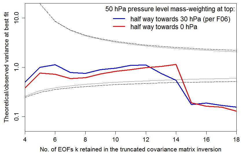
Using the F06 50 hPa level weighting, at kua = 13 the AT99 test is satisfied (although less well than at kua = 12), and the likelihood surface is more similar to that – using the same weighting – at kua = 12 than to that at kua = 14.

Upper air diagnostic likelihood surfaces
The following plots show what the upper air diagnostic likelihood consistency surface looks like in {Seq, Kv} space using the F06 50 hPa level weighting, at successively kua = 12, kua = 13 and kua = 14. Faer  has been integrated out, weighted by its marginal PDF as inferred from all diagnostics. The surface is for the CDF, not the PDF. It shows how probable it is that the upper air diagnostic r2 value at each {Seq, Kv} point could have arisen by chance, given the estimated noise covariance matrix. Note that the orientation of the axes is non-standard.

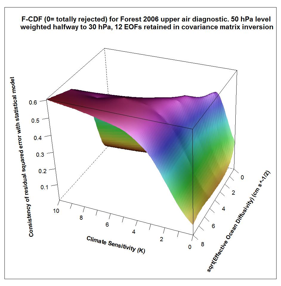
Notice that the combination of high climate sensitivity but fairly low ocean diffusivity is effectively ruled out by the kua = 12 likelihood surface, but not by the kua = 14 surface nor (except somewhere below sqrt(Kv) = 2) by the kua = 13 surface. It is the combination of high climate sensitivity but moderately low ocean diffusivity that the F06 surface and deep ocean diagnostics, acting together, have difficulty well-constraining. So the failure of the upper air diagnostic to do so either fattens the upper tail of the climate sensitivity PDF.

Why didn’t the Forest 2006 upper air r2 values reflect kua = 14, as used?
I couldn’t understand why, although F06 used kua = 14, the pattern of its computed r2 values, and hence the likelihood surface, were quite different from those that I computed in R from the same data. Why should the F06 combination of kua = 14 and 50 hPa level weighting produce one answer when I computed the r2 values in R, and a completely different one when computed by F06’s code? Compounding the mystery, the values produced by the F06 code seemed closely related to the kua = 13 case.

I could explain why each F06 r2 would only be only 80% of its expected value, because the code F06 used was designed for a different situation and it divides all the r2 values by 1.25. The same unhelpful division by 1.25 arises in F06’s computation of the r2 values for its surface diagnostic.  But even after adjusting for that, there were large discrepancies in the upper air r2 values. I thought at first that it might be something to do with IDL, the rather impenetrable language in which all the F06 code is written, having vector and array indexing subscripts that start at 0 rather than, as in R, at 1. But the correct explanation was much more interesting.

A missing data mask is generated as part of the processing of the observational data, based on a required minimum proportion of data being extant. That mask may have been used to mark what points should be treated as missing in the (initially complete) control data, when processing it to give changes from the mean of each twenty year period to the mean of a ten year period starting 25 years later. In any event, the values of the 80–85°N latitude band, 150 and 200 hPa level diagnostic variables, along with the variables for a lot of other locations, are marked as missing in the processed control data temperature changes matrix, by being given an undefined data marker value of ‑32,768°C. Such use of an undefined data marker value is common practice for external data, although not being an IDL acolyte I was initially uncertain why it was employed within IDL. It turns out that, when the code was written, IDL did not have a NaN value available.

Rogue undefined data maker values
Variables in the processed control data are then selected using a missing values mask derived from the actual processed observational data, which should eliminate all the control data variables with ‘undefined data’ marker values . Unfortunately, it turns out that the two 80–85°N latitude band control data variables mentioned, unlike all the other control data variables marked as missing by having ‑32,768°C values, aren’t in fact marked as missing in the processed observational data. So they get selected from the control data along with the valid data. I think that the reason why those points aren’t marked as missing in the observational data could possibly be linked to what looks to me like a simple coding error in a function called ‘vltmean’, but I’m not sure.  (All the relevant data and IDL code can be downloaded as large (2 GB) file archive GRL06_reproduce.tgz here.)

So, the result is that the ‑32,768°C control data marker values for the 80–85°N latitude band, 150 and 200 hPa pressure levels get multiplied by the cosine of 82.5° (the mid-point of the latitude band) and then by pressure-level weighting factors of respectively 0.05 and 0.075, to give those variables weighted values of ‑213.854°C and ‑320.781°C for all rows of the final, weighted, control data matrix.  Here’s an extract, at the point it is used to compute the whitening transformation, from the first row of the weighted control data matrix, CT1WGT, resulting from running the F06 IDL code, with the rogue data highlighted:

-0.0013 -213.8540   0.0127    0.0094     0.0051     0.0047     0.0056     0.0024     0.0005          0.0011
0.0038       0.0115     0.0125     0.0058     0.0060    0.0046      0.0030    0.0016     0.0000        -0.0002
0.0036       0.0077    0.0069     0.0001   -0.0047    -0.0060    -0.0067    -0.0050    -0.0030    -320.7810

I should say that I have been able to find this out thanks to considerable help from Jonathan Jones, who has run various modified versions of the F06 IDL code for me. These output relevant intermediate data vectors and matrices as text files that I can read into R and then manipulate.

Why does the rogue data have any effect?
Now, the control data contamination with missing data marker values doesn’t look good, but why should it have any effect? A constant value in all rows of a column of a matrix gives rise to zero entries in its covariance matrix, and a corresponding eigenvalue of zero, which – since the eigenvalues are ordered from largest to smallest – will result in that eigenfunction being excluded upon truncation.

But that didn’t happen. The reason is as follows. F06 used existing Detection and Attribution (D&A) code in order to carry out the whitening transformation – an IDL program module called ‘detect’.  That appears to be a predecessor of the standard module ‘gendetect’, Version 2.1, available at The Optimal Detection Package Webpage, which I think will have been used for a good number of published Detection and Attribution studies. Now, neither detect nor gendetect v2.1 actually carries out an eigendecomposition of the weighted control data covariance matrix.  Instead, they both compute the SVD of the weighted control data matrix itself. If all the columns of that matrix had been centred, then the SVD eigenvalues would be the square roots of the weighted control data sample covariance matrix eigenvalues, and the right singular vectors of the SVD decomposition would match that covariance matrix’s eigenvectors.

However, although all the other control data columns are pretty well centred (their means are within ± 10% or so of their – small – standard deviations), the two columns corresponding to the constant rogue data values are nothing like zero-mean. Therefore, the first eigenfunction  almost entirely represents a huge constant value for those two variables, and has an enormous eigenvalue. The various mean values of other variables, tiny by comparison, will also be represented in the first eigenfunction. The reciprocal of the first eigenvalue is virtually zero, so that eigenfunction contributes nothing to the r2 values. The most important non-constant pattern, which would have been the first eigenfunction of the covariance matrix decomposition, thus becomes the second SVD eigenfunction. There is virtually perfect equivalence between the eigenvalues and eigenvectors, and thus the whitening factors derived from them, of the SVD EOFs 2–14 and (after taking the square root of the eigenvalues) those of the covariance matrix eigendecomposition EOFs 1–13. So, although F06 ostensibly uses kua=14, it effectively uses kua =13. Mystery solved!

Concluding thoughts
It’s not clear to me whether, in F06’s case, the combination of arbitrary marker values incorrectly getting through the mask and then dominating the SVD had any further effects. But it is certainly rather worrying that this could happen. Is it possible that, without centring, the means of a control data matrix could give rise to a rogue EOF that did affect the r2 values, or otherwise materially distort the EOFs, in the absence of any masking error? If that did occur, might the results of some D&A studies be unreliable? Very probably not in either case. However, it does show how careful one needs to be with coding, and importance of making code as well as data available for investigation.

There was actually a good reason for use of the SVD function (from the related PV-wave language, not from IDL itself) rather than the IDL PCA function, which despite its name does actually compute the covariance matrix. Temperature changes in an unforced control run have a zero mean expectation, provided drifting runs are excluded. Therefore, deducting the sample mean is likely to result in a less accurate estimate of the control data covariance matrix than not doing so (by using the SVD eigendecomposition, or otherwise). However, the downside is that if undefined data marker values are used, and something goes wrong with the masking, the eigendecomposition will be heavily impacted. Version 3.1 of gendetect v3.1 does use the PCA function, so the comments in this post are not of any possible relevance to recent studies that use the v3.1 Optimal Detection Package code. However, I suspect that Version 2.1 is still in use by some researchers.

So, the lesson I draw is that use within computer code of large numbers as marker values for undefined data is risky, and that an SVD, rather than a eigendecomposition of the covariance matrix, should only be used to obtain eigenvectors and eigenvalues if great care is taken to ensure that all variables are in fact zero mean (in population, expectation terms).

Finally, readers may like to note that I had a recent post at Climate Etc, here, about another data misprocessing issue concerning the F06 upper air data. That misprocessing appears to account for the strange extended shoulder between 4°C and 6°C  in F06’s climate sensitivity PDF, shown below.

Nic Lewis