A guest post by Nic Lewis
When the Lewis & Crok report “A Sensitive Matter” about climate sensitivity in the IPCC Fifth Assessment Working Group 1 report (AR5) was published by the GWPF in March, various people criticised it for not being peer-reviewed. But peer review is for research papers, not for lengthy, wide-ranging review reports. The Lewis & Crok report placed considerable weight on energy budget sensitivity estimates based on the carefully considered AR5 forcing and heat uptake data, but those had been published too recently for any peer reviewed sensitivity estimates based on them to exist.
I am very pleased to say that the position has now changed. Lewis N and Curry J A: The implications for climate sensitivity of AR5 forcing and heat uptake estimates, Climate Dynamics (2014), has just been published, here. A non-paywalled version of the paper is available here, along with data and code. The paper’s results show the best (median) estimates and ‘likely’ (17–83% probability) ranges for equilibrium/effective climate sensitivity (ECS) and transient climate response (TCR) given in the Lewis & Crok report to have been slightly on the high side.
Our paper derives ECS and TCR estimates using the AR5 forcing and heat uptake estimates and uncertainty ranges. The analysis uses a global energy budget model that links ECS and TCR to changes in global mean surface temperature (GMST), radiative forcing and the rate of ocean etc. heat uptake between a base and a final period. The resulting estimates are less dependent on global climate models and allow more realistically for forcing uncertainties than similar estimates, such as those from the Otto et al (2013) paper.
Base and final periods were selected that have well matched volcanic activity and influence from internal variability, and reasonable agreement between ocean heat content datasets. The preferred pairing is 1859–1882 with 1995–2011, the longest early and late periods free of significant volcanic activity, which provide the largest change in forcing and hence the narrowest uncertainty ranges.
Table 1 gives the ECS and TCR estimates for the four base period – final period combinations used.

Table 1: Best estimates are medians (50% probability points). Ranges are to the nearest 0.05°C
AR5 does not give a 95% bound for ECS, but its 90% bound of 6°C is double that of 3.0°C for our study, based on the preferred 1859–1882 and 1995–2011 periods.
Considerable care was taken to allow for all relevant uncertainties. One reviewer applauded “the very thorough analysis that has been done and the attempt at clearly and carefully accounting for uncertainties”, whilst another commented that the paper provides “a state of the art update of the energy balance estimates including a comprehensive treatment of the AR5 data and assessments”.
Earlier sensitivity studies based on observed warming during the instrumental period (post 1850) have generally used forcing estimates derived from one or more global climate models (GCMs), particular published studies and/or the forcing estimates given in AR4 – which were only for a single year. Our paper appears to be the first to use the comprehensive set of forcing time series and uncertainty ranges provided in AR5. They are based on careful assessments of forcing estimates from various published studies, and are likely to become widely used in observationally-based sensitivity studies.
There is thus now solid peer-reviewed evidence showing that the underlying forcing and heat uptake estimates in AR5 support narrower ‘likely’ ranges for ECS and TCR with far lower upper limits than per the AR5 observationally-based ‘likely’ ranges of: 2.45°C vs 4.5°C for ECS and 1.8°C vs 2.5°C for TCR. The new energy budget estimates incorporate the extremely wide AR5 aerosol forcing uncertainty range – the dominant contribution to uncertainty in the ECS and TCR estimates – as well as thorough allowance for uncertainty in other forcing components, in heat uptake and surface temperature, and for internal variability. The ‘likely’ ranges they give for ECS and TCR can properly be compared with the AR5 Chapter 10 ‘likely’ ranges that reflect only observationally-based studies, shown in Table 1. The AR5 overall assessment ranges are the same.
The CMIP5 GCMs used for AR5 all have ECS values exceeding 2°C, whereas 70% of our preferred main results ECS probability lies below that level, and over 90% lies below the 3.2°C mean ECS of CMIP5 models. The 33 CMIP5 models with suitable archived data show TCR values exceeding our preferred best estimate of 1.33°C in all but one case, with an average TCR exceeding the top of our 1.8°C ‘likely’ range.
The Otto et al 2013 energy budget study (of which I was an author) used ensemble mean forcing data derived from simulations by CMIP5 climate models, with an adjustment reflecting the difference between CMIP5 models’ aerosol forcing and the AR5 best estimate. Our preferred TCR best estimate exactly matches the lowest uncertainty Otto et al estimate, that using a 2000–09 final period; their estimate using a long 1971–2009 period was almost the same. The Otto et al ECS best estimates based on data for those two periods are slightly higher than ours based on 1995–2011 and 1987–2011 data. For 2000–2009 that is mainly because heat uptake estimates over that period vary considerably and Otto et al used a high estimate. For 1970–2009 it is likely mainly due to a large mismatch in volcanic forcing with the common base period of 1860–79 used for all its estimates.
Our preferred ECS and TCR estimates are closely in line with those from other recent instrumental-observation studies based on warming over the bulk of the instrumental period that use spatiotemporal temperature data (not just GMST) to make their own estimate of aerosol forcing, and do not use a prior distribution that strongly pushes their ECS or TCR estimate towards values above where the data fits best. Those studies are: Aldrin et al. (2012), Ring et al. (2012), Lewis (2013) and Skeie et al. (2014).
Some recent studies (e.g., Huber and Knutti, 2014) seek to imply that ECS and/or TCR estimates in line with ours and those in the above-mentioned studies, which point to CMIP5 GCMs being oversensitive, are strongly influenced by the low increase in surface warming this century. Rogelj et al (2014) named four studies in this regard (Schmittner et al 2011, Aldrin et al 2012, Lewis 2013 and Otto et al 2013). The claim is factually incorrect in respect of all four studies. And for our study, ECS and TCR estimates using final periods from 1971 or 1987 to 2000, 2001, 2002 or 2003 differ very little from those using data to 2011.
It has been claimed that incomplete coverage of high-latitude zones in global temperature datasets biases down their estimate of the rate of increase in GMST. However, over the long periods involved in this study there is no evidence of any such bias. The increase in GMST per the published HadCRUT4v2 global dataset, used in the study, exceeds rather than underestimates the area-weighted average of the calculated increases for ten separate latitude zones, which method gives a full weighting to each zone.
Scientists who work on or with global climate models (GCMs) tend to be suspicious of observationally-based ECS and TCR estimates that lie well below the values indicated by most GCMs. One of their arguments is that most ECS estimates based on warming during the instrumental period are actually of effective climate sensitivity, which reflects climate feedbacks during the period studied, and that many GCMs show feedbacks changing and effective climate sensitivity increasing over time, so that energy budget and other instrumental observation-based estimates of ECS will be too low.
However, it is standard to estimate the equilibrium sensitivity of coupled GCMs from regressing radiative imbalance on GMST over a 150 year simulation involving an artificial scenario with an abrupt quadrupling of CO2 concentration. The vast majority of such regression plots show no evidence of the strength of climate feedbacks changing measurably over time, apart from (for about half the GCMs) during the first year or two when the climate system is undergoing very rapid adjustment to the quadrupling of CO2. If such behaviour in that period reflects reality, there would be an effect on the relationship of energy budget ECS estimates to the regression-based estimate of equilibrium sensitivity, but it would be extremely small and possibly negative.
It is claimed in a model-based study (Shindell, 2014) that spatially inhomogeneous forcings, principally from aerosols and ozone, lead to substantial underestimation of TCR by global energy budget and similar methods, with the levelling off of aerosol forcing in recent decades exacerbating the underestimation. ECS estimation could also be affected. Whilst the underlying arguments may well be valid, based on real world data their effects on TCR estimation appear minor – on my rough calculations, only a few percent.
Going the other way, AR5 assesses the overall effects on forcing of land use change as equally likely to be positive or negative, but its forcing estimates only include the negative albedo effect. If land use forcing is centred at zero, but with doubled uncertainty, reflecting AR5’s assessment, the preferred period combination best estimate for ECS drops to 1.54°C, with a 95% bound of 3.5°C. The TCR best estimate falls to 1.27°C, with a 95% bound of 2.3°C.
The study does not assume any possible contribution to the increase in GMST from indirect solar influences not allowed for in the AR5 forcing estimates, or from natural internal climate variability affecting ocean heat uptake and/or forcing.
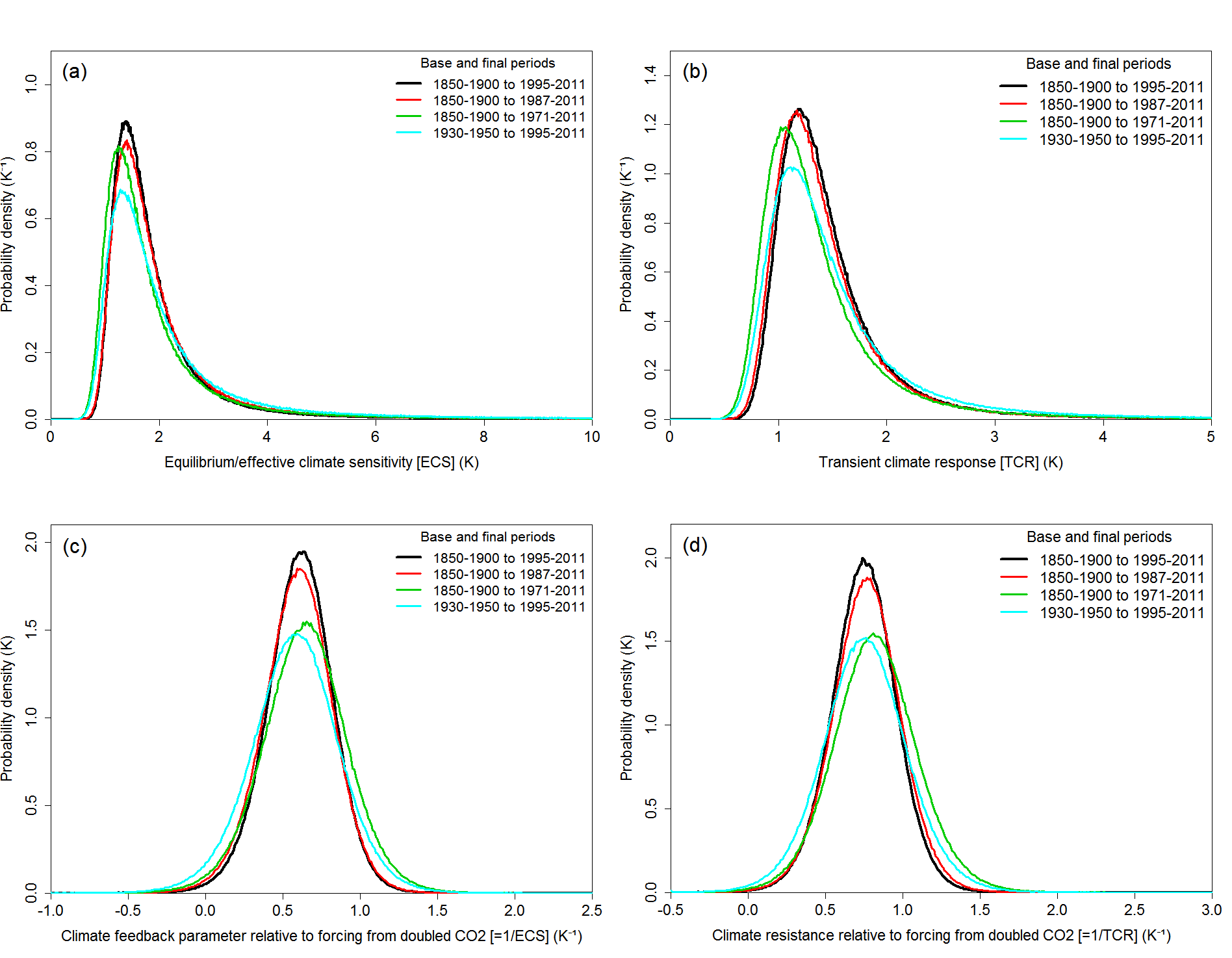
Figure 1: Estimated PDFs for ECS and TCR, and their reciprocals, for the four period combinations
The paper’s ECS and TCR estimates, and the uncertainty associated with them, could also be presented in the form of probability density functions, as in panels a and b of Figure 1. The PDFs are skewed due principally to the dominant uncertainty, that in forcing, affecting the denominator of the fractions used to estimate ECS and TCR.
Skewed PDFs can be misleading. With an unchanged best estimate (the median or 50% probability point, typically identical or very close to the estimate obtained disregarding uncertainties), the PDF mode (location of its peak) moves away from the best estimate as data uncertainties increase. Reparameterizing ECS and TCR as their reciprocals (being the climate feedback parameter in the case of ECS, ignoring uncertainty in ), as in the lower panels c and d of Figure 1, results in much less skewed PDFs and avoids the mode shifting misleadingly as the width of the PDF varies. If these reciprocal parameterisations had been used in climate science, much of the misunderstanding about Bayesian inference and choice of priors that has held back progress in observationally-based estimation of ECS would likely not have occurred. When estimation errors for a parameter have fixed, symmetrical Gaussian or similar distributions – as those in panels c and d approximately do – then few people would normally dispute use of a uniform prior for it. The PDFs for ECS and TCR shown in panels a and b – which embody highly non-uniform priors – can be obtained from those for 1/ECS and 1/TCR in panels c and d by applying the standard change-of-variables formula.
.
Nicholas Lewis
Postscript (dated 24 September 2014)
A commenter asked for an extended table giving comparisons with other recent studies as well. Such a table follows. The numbers are from my own calculations. Two estimates are given for Aldrin et al (2012), one based on a uniform-in-ECS prior and the other on a uniform-in-1/ECS prior. I believe the 1/ECS prior to provide more objective ECS estimates. The TCR estimates for Lewis (2013) are derived from its ECS and ocean effective diffusivity estimates using an empirical formula. The Skeie et al (2014) TCR estimates are based on a distribution fitted to the mean and range given in the paper. Ring et al (2012) did not give any uncertainty ranges and so is not included. Its ECS best estimates varied from 1.4 to 2.0 C depending on surface temperature dataset used. These are the only other recent studies that form their own inverse estimate of aerosol forcing using data resolved at least hemispherically (or use an estimate thereof that is consistent with the AR5 best estimate) and which do not use a prior distribution that strongly pushes their ECS or TCR estimate towards substantially higher values than found in the new paper. (Full references for these various studies are given in the paper.)

I would also like to clarify, in relation to the Lewis and Crok report “A Sensitive Matter”, that (as with all GWPF reports) it was sent for comment and review to all members of the GWPF Academic Advisory Council. Accordingly, whilst it was not published in a peer reviewed journal, the criticism it received for not being peer-reviewed was inaccurate. It had undergone peer review, albeit under a different (but arguably typically more rigorous) procedure from that of a journal.


47 Comments
Congrats on the publication!
Congratulations Nic.
It would be helpful to see an extended version of your table, to include summaries of the results from other recent papers (Ring, Aldrin etc) for comparison.
Nic, thanks for the extended summary-comparison table, that’s very helpful.
Wow. What a week in the climate blogosphere, in gatherings of sceptics, in fruitful confidential discussions with official climate scientists and, now, in peer-reviewed publication, with open code and data. Well done Judy and Nic.
Interesting to contrast your Table 1 values with those of AR5 WG1 Table 9.5 (CMIP5 GCMs).
ECS: 18 of 23 are above your 83% value of 2.45. The remaining 5 are all above your best estimate of 1.64. [Well above, being in the range of 2.1 to 2.4.]
TCR: 14 of 30 are above your 83% value of 1.8, plus 2 at 1.8; 11 more above your best estimate of 1.33. 3 are below best estimate and above your 17% point (1.05).
A similar comparison to AR5 WG1 Table 9.6 (EMICs)–
ECS: 10 of 14 above the 83% value (2.45); remaining 4 above the best estimate (1.64).
TCR: 8 of 15 above the 83% value (1.8); 5 more above best estimate (1.33); 1 below best estimate but above 17% value (1.05); 1 below 17% value (1.05).
It is a real and rare pleasure to read a climate piece that systematically addresses possible limitations and counter arguments and does so in a way that encourages further discussion and debate. This is the way I thought the hard sciences were supposed to operate. Outstanding job.
Congratulations Nic. The implications are vast leading into Paris 2015.
Now we know why AR5 produced no onservational best estimate from their own best T, Q, and F estimates. Falsifies CMIP5 and cancels the notion of any climate crisis.
Your paper is more than the end of the beginning. More like the beginning of the end.
In order for this to be a real canceling of the “notion of any climate crisis”, wouldn’t these ECS values have to themselves change over time, particularly with increasing CO2 concentration.
For example, even if ECS is, say 1.5°C per 2xCO2 — aren’t we heading for well more than 2xCO2 in the future … That corresponding magnitude of warming certainly seems like it will be eventually long without precedent, rather than debatably unprecedented, yes?
Not necessarily. We are at about 400 ppm right now, going up about 2 ppm per year. That works out to about two centuries to double from now at current rates. Most likely we mostly stop burning fossil fuels way before 200 years so this should enormously reduce the amount of co2 that man releases. As far as the co2 released by nature, Que sera, sera.
The doubling baseline is to pre-industrial averages, is it not? Also, given our very slow rate of energy decarbonisation relative to our rate of total energy growth (in line with GDP), and given the long atmospheric life cycle of carbon, wouldn’t your comments seem overly rosy?
I’m not sure that erring on the rosier side in terms of ECS uncertainty should be combined with erring on the rosier side of renewable energy progression. Naturally such an exercise would yield a doubly-acceptable outcome with minimal “forced effort” on the part of nations… but wouldn’t it also open up the possibility that the non-rosy combination is also there..? Namely, higher ECS and slower progression to full renewables…
To re-ask Salamano’s question, is TCR/ECS based on a doubling from WHEREVER we start – (280 or 400), or ONLY when starting from 280?
From a linguistic clarity perspective, if it is only from 280ppm, it seems specious to talk about “doubling” at all, instead of just saying 560ppm.
I wonder why they do not make this perfectly clear – since the ramifications of the difference are so dramatic. Their lack of clarity is frustrating.
For example, In this table from AR5-WG1 (12-25)

they state that they base future temperature ranges on a 1968-2005 timeframe.
However, their projected temperature increases for RCP4.5 (538ppm) at 300 years shows a range from 1.4-3.5. This is less than the ECS for a doubling of CO2 from 280pmm. However, their projection for RCP4.5 at 100 years matches the TCR for doubling almost precisely (1.1-2.6).
Are they saying (in this table) that they expect temperature to rise 1.4 +/- 0.3 in the next 50 years – then only 0.4 in the following 50? Or do they mean that since temperature from 1900-2005 has already raised 1.4 degrees – we have already seen most of the heat rise we have already seen? How do we make sense of this table?
I suppose expecting clarity and precision/consistency among the various parts of WG1 (given the scope of the project or the political intentions of its authors, or both) is naive on my part, but I don’t understand how they can publish it with a straight face. My professors would have rejected this paper and shamed me for not doing better.
It seems that they would make the basic science paper WG1 clear – since it is what everything else is based on. It is frustrating.
bad link – sorry

Wow! Nice work Nic and Judy! So great you two were able to work together on this. And lets not forget Steve Mc who has been leading the way all these years. You folks are incredible!
And this goes nicely with Jean S. post on Black Tuesday, recounting in summary what Steve Mc and CA pioneered.
Nic,
I here cross post a comment I made at Judith’s blog:
Congrats. Very nice paper.
I was myself already using AR5 forcing estimates and heat uptake data to estimate ECS, using the 1850 to 2011 period. I got a most probable value of 1.55C/doubling, a 17% to 83% range of 1.41C to 3.27C/doubling, and a 5% to 95% range of 1.18C to 6.2C/doubling… not far from your values (but I assumed a little higher total heat accumulation, including deep ocean uptake equal to 10% of the 0-2000M value, and some additonal heat for ice melt and land mass warming). The median sensitivity I got was 1.97 C/doubling.
One interesting point I noted (and your paper confirms) is that if you reduce the forcing uncertainty from the IPCC level, but don’t change the IPCC’s best estimate of forcing, the most probable value of ECS increases very slightly, but the high sensitivity tail (eg total probability for sensitivity above 3.5C per doubling) almost disappears. This points to the importance of narrowing the uncertainty in forcing to more accurately define the high sensitivity tail, and so better constrain which GCM’s generate plausible diagnosed sensitivities and which do not. The overall uncertainty is dominated by direct and indirect aerosol effects… and here there is a crying need for better data. If the forcing uncertainty could be reduced by 1/2, most of the model diagnosed sensitivity values would (I think) be clearly much too high.
I suspect your paper will get some push back based on papers which claim there is a substantial difference (>~10-15%) between effective and equilibrium sensitivity (for example, Armour et al 2013), with effective sensitivity always lower than equilibrium sensitivity. My personal take is that the difference is probably quite small, and even if it is not, from a practical viewpoint, the effective sensitivity value is going to be a very good predictor of warming, at least for 100 to 150 years or so.
I’m a little confused by this statement:
“It has been claimed that incomplete coverage of high-latitude zones in global temperature datasets biases down their estimate of the rate of increase in GMST. However, over the long periods involved in this study there is no evidence of any such bias. The increase in GMST per the published HadCRUT4v2 global dataset, used in the study, exceeds rather than underestimates the area-weighted average of the calculated increases for ten separate latitude zones, which method gives a full weighting to each zone.”
There are three available datasets that go back to 1850. CW2014, Hadcrut4v2 and BEST. Both CW2014 and BEST show about 10% more warming using your preferred base and final periods (1859-1882; 1995-2011). Is the rationale for not including coverage bias or either of these datasets discussed in more detail anywhere?
With no satellites from 1850 until the later 20th century, can the C&W method really be applied with any confidence?
The question you have is whether its better to simply input the global average (a la HadCRUTv4) or whether its better to estimate temperatures geostatistically from high latitude stations (a la CW2014/BEST). We did a fair bit of cross-validation with our normal (kriged) data and conclude that it performs reasonably well (and certainly better than inputting the global average).
The HadCRUTv4 method inevitably will overestimate global temperatures in periods where the Arctic is cold and will underestimate global temperatures in periods where the Arctic is warm.
OK. Do you have enough high latitude data to make statistically confident estimates of the biases in HadCRUT4 over the whole period from 1850? I mean, do you have evidence that the true high latitude temps were biased high when the global average was 0.8C lower than today? If so, how much do you think the average temperatures were biased high in the past? I am trying to get a feel for the magnitude of the overall bias in global average you are suggesting is present in HadCRUT4.
The short answer is yes. There is plenty of data not included in HadCRUT4v2 which is for example included in BEST. I know first hand from the region where I worked the most that if you based off of HadCRUTv4 you would overestimate the air temperature compared to data which is available but has not been used by CRU because of their CAM restrictions. I tend to think that everytime people look at it with extra data you get a colder past and a warmer present in high latitude areas.
At some point the whole argument with respect to physics and Arctic Amplification has to come in as well. You could treat this a couple of ways – you could (a) assume that this is the only period where the Arctic has warmed/cooled faster than the global average; or (b) assume that when warming/cooling occurs in the Arctic it is amplified through largely albedo and vegetation feedbacks. Since we can measure that Arctic Amplification is occurring right now, and we know that it occurred as well during previous periods of warming/cooling then it is a safe bet that if your coverage of the Arctic is reduced you will miss some of it. The new international surface temperature initiative will provide further evidence of that.
“. I tend to think that everytime people look at it with extra data you get a colder past and a warmer present in high latitude areas.”
That has been my experience.
every time we add data you either get no movement or a colder past and warmer present.
Robert Way wrote:
“…Arctic Amplification is occurring right now, and we know that it occurred as well during previous periods of warming/cooling”
I am very curious as to where I can read more about previous periods of arctic amplification (is “amplification” a technically accurate term?), so if you can point me to any references, it would be greatly appreciated.
As I recall Cowtan and Way showed a faster global warming from 1997-2012 than GISS, and primarily the result of differences in the Arctic region, but when the comparison was from 1979-2012 the difference between CW and GISS trends was small. Perhaps Robert Way can enlighten use by showing the warming/cooling trends for CW versus HadCRUT4 for the various periods used in the Nic Lewis calculations – and confidence intervals for differences.
Matt Skaggs,
here are two good papers on the topic:
Miller et al. (2010). Arctic amplification: can the past constrain the future? Quatenary Science Reviews, 29: 1779-1790.
Serreze, M.C. and Barry, R.G. (2011). Processes and impacts of Arctic amplification: A research synthesis. Global and Planetary Change, 77: 85-96.
C&w should be looked at as a sensitivity. With the code
Available that should be straightforward
C&W have done an analysis using MERRA to infill that I really like. It gets around some of the issues that Robert Way was pointing out regarding the use of reanalysis products to estimates long-term trends, but where the interpolation scheme is physically based.
I would say “a 10% effect” is an exaggeration. If you’re looking at small trends that can have either sign, you should be describing it as an additive correction.
You can get a good idea of the magnitude of the correction by comparing e.g.the 10-y trends from the different reconstructions to the uncorrected HADCrut4 series:
if you look at the start of the 2007 series, it crosses through zero and the raw HADCrut4 series is negative.
My point is, does it really make sense to describe the effect of the correction as “XX% warmer”?
Sorry garbled this:
“if you look at the start of the 2007 [for the MERRA] series, it crosses through zero and the raw HADCrut4 series is negative.'”
still I think it makes sense to do the study with alternative temp series
Sorry, Carrick, I did not read your post before posting mine and so perhaps you have presented at least some of what I wanted. Are the HadCRUT4 + xxx series actually based on CW temperature data sets? I thought a previous Nic Lewis study or his discussion about it gave results using GISS – although GISS goes back only to 1880.
Robert Way
“There are three available datasets that go back to 1850. CW2014, Hadcrut4v2 and BEST. Both CW2014 and BEST show about 10% more warming using your preferred base and final periods (1859-1882; 1995-2011). Is the rationale for not including coverage bias or either of these datasets discussed in more detail anywhere?”
Our paper uses AR5 forcing and heat uptake data and, consistently, considers the three GMST datasets cited in AR5. CW2014 and BEST were not so cited.
IMO your comment about BEST is misleading. The difference in its warming between 1859-1882 and 1995-2011 with HadCRUT4v2 appears to have nothing to do with coverage bias. In the light of my analysis finding that the increase in GMST per the published HadCRUT4v2 global dataset exceeds the area-weighted average of the calculated increases for ten separate latitude zones, that seems unsurprising.
BEST has two GMST versions, with differing treatment of sea ice temperature. One of the versions produces an almost identical (<1% different) increase to HadCRUT4v2, the other a 9% higher increase. Neither HadCRUT4 or NOAA/NCDC's MLOST datasets appear to adopt a treatment of sea ice temperature corresponding to the faster warming version of BEST.
I haven't studied Cowtan & Way 2014 in any detail. It is accordingly unclear to me whether its method of reconstructing data in unobserved regions is substantially superior to those used by MLOST, GISS or JMA, even assuming that it is desirable to carry out such infilling. In any event, I prefer GMST datasets that avoid use of data containing non-overlapping records of different stations that have been stitched together without homogenisation.
“I haven’t studied Cowtan & Way 2014 in any detail. It is accordingly unclear to me whether its method of reconstructing data in unobserved regions is substantially superior to those used by MLOST, GISS or JMA, even assuming that it is desirable to carry out such infilling.”
Then perhaps its time you read CW2014 and the 3 subsequent updates online. If you did you would see that cross-validation tests, tests against local out-of-sample data, reanalysis data, satellite data (AIRS, AVHRR/MODIS skin temperature) all show that the method adopted by CW2014 and BEST (sea-ice as land) outperform other methods. Simmonds and Pauli (In press) QJRMS have look in detail at our record as well.
Implicitly by using Hadcrut4 or MLOST you infill the global average – try that with cross-validation and you see clearly how that method introduces increasing bias with higher latitude. MLOST has even less high latitude coverage than CRU.
The differences between BEST and CW2014 with GISS are more interesting. GISS uses GHCN which has less data than CRU in the Arctic and also shows evidence of downward homogenization adjustments that lead to recent Arctic trends that are inconsistent with satellite data. (as seen in one of our updates).
If you haven’t read the papers or tested the methods then its hard to accept your reasoning for not including. Your intuition is not the same as actually looking at the data. I just do not understand how from a communications standpoint it makes sense to even open yourself up to the cherry-picking accusation from those you’re trying to convince of your papers credibility.
It’d take more than a few hours to parse through your code and test it out – but when I get time to commit to that I will, but in the meantime you’re welcome to provide that information.
To be fair, using the datasets in AR5 isn’t exactly arbitrary or cherry picking. However, I think you’ve somewhat convincingly shown that your method is more accurate… and that, whether one agrees with the preceding sentence or not, re-doing the Lewis&Curry(2014) analysis with your data could not hurt anything and could lead to a lot of learning.
Robert Way,
On the contrary, using temperature datasets not referenced in AR5 would actually have served to open the authors up to accusations of cherry-picking. Considering the sheer amount of effort put forth into AR5, it seems far more useful to maintain the same foundation and context as AR5.
Should your method be shown to be superior, I’m sure it will be included in the next AR.
Nic (& Judith):
Thanks for this, and congrats on the publication!
You should be sure to send a copy to Steven E. Koonin, https://en.wikipedia.org/wiki/Steven_E._Koonin
He remarked, in his recent WSJ essay
http://online.wsj.com/articles/climate-science-is-not-settled-1411143565 “Climate Science Is Not Settled” that
“Today’s best estimate of the sensitivity (between 2.7 degrees Fahrenheit and 8.1 degrees Fahrenheit) is no different, and no more certain, than it was 30 years ago. And this is despite an heroic research effort costing billions of dollars.”
Good to see you two answering this problem, and on a considerably lower budget!
Cheers — Pete Tillman
Professional geologist, amateur climatologist
Mt. Tillman: absolutely wrt Koonin. The fact that now he has recanted, or at least come clean, about his doubts indicates the extraordinary level of green orthodoxy imposed on the US DOE and other agencies by ruthless hard left enforcers such as Holdren and Podesta at the white house. Koonin has the scientific credentials but even he was intimidated. He must now, however, be supported as the inevitable attacks from Romm and others will ensue. In this vein this new paper is extremely important.
nope. not saturated
Enquiring minds politely ask for more than a 3 word answer…
OHC discussion –
“Gregory et al (2013) …However the CCSM4 model has TCR and ECS values of 1.8K and ca. 3.0K that are some 35-85% higher than the best estimates for those parameters arrived at in this study. We therefore take only 60% of the base period heat uptake estimated from the Gregory et al (2013) simulations…”
Does this need to be justified further, and what is the effect on the results if 100% of Gregory et al is used?
(noted also the increased standard error)
You can work out from Table 2 in the paper what the effect on deltaQ of using 100% rather than 60% of the Gregory et al estimate for the base period heat uptake is. For the preferred results, which use 1859-82, doing so reduces deltaQ by 0.1 W/m2 (-40%/60% * 0.15). As stated in section 6, the effect of that is shown by the “2011 ERF_LUC recentred on zero line” of Table 5. The best ECS estiamtes becomes 1.54 C, and that for TCR 1.27 C. The upper uncertainty bounds show greater declines.
I guess the irony here is that the “it’s worse than we thought” crowd now actually have reason to fear that things, are, indeed, worse than they thought.
I am not pretending to have any understanding of this paper to make a comment on it but Richard Betts made a comment at Bishop Hill, on another topic, about observational estimates like this being made under a lower amount of forcing that can be expected later. My understanding of this comment is that ECS and TCS are not constants but will vary with the amount of CO2 in the atmosphere. GCMs are the only way to overcome this possible limitation of observational studies.I hope that this is a correct understanding of the comment and that I have not distorted Betts’ comment too much.
Would Nic Lewis care to comment on this?
I don’t know what exactly Richard Betts said, but there is little evidence from GCMs that ECS or TCR vary much if at all with CO2 levels, at least until you get some way past 4x preindustrial (PI) levels (circa 1200 ppm – 3x current levels). In fact, ECS – the equilibrium warming for a doubling of CO2 – in CMIP5 models and other coupled GCMs is usually estimated as half of their simulated response to a quadrupling of CO2 levels. That procedure assumes the constancy of ECS with CO2 levels, which is indeed demonstrated by most if not all GCMs.
If there’s little change in ECS or TOR with CO2 levels, then
Aren’t we still looking at some 2x-3x+ of CO2 levels from pre-industrial times through to 2100 … Meaning, global temperature rising 2.5F to 6F over those days..? Isn’t that range also problematic for a pure adaptation/un-coerced mitigation path?
Nic Lewis has previously made projections for 2100 using the Otto2013 TCR range, which is not exactly the same as that of Lewis & Curry, but fairly close. (See Nic’s update above for comparison.) For the RCP8.5 scenario, he obtained a best estimate of around 3 K increase relative to pre-industrial. For the (IMO, the more realistic) RCP6.0 scenario, one would expect proportionately less warming, perhaps 2 K. (Equivalent to an increase from today’s temperatures of about 1.2 K.]
Is that problematic? Not sure there’s an objective answer to that question.
Thanks.
I guess that’s for all the policy wonks and politicians to step in and decide…
I’m guessing there’s always a fanciful nostalgia for the days of old as always being perfect, and all endangered species need special preservation, etc… But I’d also go so far as to say that for the globe (or especially higher latitudes) pre-industrial conditions would be determined as ‘too cold’ under a number of optimums. However, if that meant some tropical island in the Pacific with a small indigenous population had a few feet more of shore, to them it’s better for 45N to have crappier winters, etc.
In that case they’re losing…
“[T]hat’s for all the policy wonks and politicians to step in and decide…”
Actually, it should be for us, the voting public, to decide. Not that we are necessarily less self-interested. But we might be less inclined to be concerned with our political profile (for rising pols) or legacy (for those already at the top). Or to make decisions on century-scale time horizons in the belief that predictions so far ahead — climatic, economic, or political — are as accurate as astronomical predictions. The policy wonks, who deal in spreadsheets, seem rather more inclined to rely upon these numbers because they’re “objective”. But as has been said before, prediction is very difficult, especially about the future.
Excellent paper Nic and Judy! Nic, as you may know I get numbers very close to yours with a slightly different method. (The method I’m using employs a best-fit analysis considering all years since 1850). I have, in addition, just recently looked at the potential effect of including an allowance for the possible effect of a natural temperature oscillation with an unknown source, but with a period of about 60 years that is implied by global temperature observations. The analysis consideres the possibility of either an externally forced oscillation that changes the TOA radiation balance (maybe some unknown solar amplification factor?) or a long-period natural oceanic oscillation that simply re-distributes ocean heat to or from the surface without a major change in net ocean heat content. Both these changes reduce the estimated ECS, with the ocean-heat redistributation yielding the greatest effect, giving an ECS of a little over one degree C, though the externally forced option is probably a little more consistent with ocean heat content observations. Either of these assumptions holds out the substantial prospect of limiting the GHG warming to less than the magical two degrees C with emissions constrained by nothing more than the finite nature of fossil fuel reserves and resources.
I read that Lewis is an independent climate scientist. How does one become an independent scientist? How do you get paid or make a living at it?
Steve: he’s made money previously in his career and is doing it of interest.
15 Trackbacks
[…] UPDATE: The CA post is up at https://climateaudit.org/2014/09/24/the-implications-for-climate-sensitivity-of-ar5-forcing-and-heat-… […]
[…] The implications for climate sensitivity of AR5 forcing and heat uptake estimates (Climate Audit) […]
[…] The implications for climate sensitivity of AR5 forcing and heat uptake estimates (Climate Audit) […]
[…] So much of the IPCC argument is based on uncertainty. Nic Lewis has been working rather tirelessly on improving climate science’s understanding of the observation based magnitude of warming from CO2. This time he teamed up with Judith Curry and published a new paper establishing a far tighter uncertainty range for climate sensitivity to CO2 based warming. The answers they show are substantially lower than the IPCC model based estimates and in my opinion substantially more credible. See Nic’s article describing their results at climate audit here. […]
[…] and a much more thorough description of the research, author Nic Lewis takes you through the paper (here) has made a pre-print copy of the paper freely available […]
[…] and a much more thorough description of the research, author Nic Lewis takes you through the paper (here) has made a pre-print copy of the paper freely available […]
[…] a blog post explaining the study, Lewis stressed their results “are less dependent on global climate models” than other […]
[…] and a much more thorough description of the research, author Nic Lewis takes you through the paper (here) has made a pre-print copy of the paper freely available […]
[…] Earth & not forget our save-the-worlder’s moving tipping points too. Future temps are now decreasing; Antarctic ice is again at record highs; Arctic ice is increasing & Ozone […]
[…] are excerpt from Nic Lewis’ blog post at ClimateAudit on […]
[…] of equilibrium climate sensitivity is 1.64 degrees C. Lewis describes the paper’s methodology here, and you can follow the link to the paper and read it for […]
[…] A guest post by Nic Lewis. When the Lewis & Crok report “A Sensitive Matter” about climate sensitivity in the IPCC Fifth Assessment Working Group 1 report (AR5 … more… […]
[…] a paper published last year (Lewis & Curry 2014), discussed here, Judith Curry and I derived best estimates for equilibrium/effective climate sensitivity (ECS) and […]
[…] AR5 kom ut at forskningen på dette feltet har gjort fremskritt. Nicholas Lewis publiserte ifjor en rapport sammen med Judith Curry hvor man gjorde et beste estimat for equilibrium/effective climate […]
[…] a paper published last year (Lewis & Curry 2014), discussed here, Judith Curry and I derived best estimates for equilibrium/effective climate sensitivity (ECS) and […]