A guest post by Nicholas Lewis
In a paper published last year (Lewis & Curry 2014), discussed here, Judith Curry and I derived best estimates for equilibrium/effective climate sensitivity (ECS) and transient climate response (TCR). At 1.64°C, our estimate for ECS was below all those exhibited by CMIP5 global climate models, and at 1.33°C for TCR, nearly all. However, our upper (95%) uncertainty bounds, at 4.05°C for ECS and 2.5°C for TCR, ruled out only a few CMIP5 climate models. The main reason was that they reflected the AR5 aerosol forcing best estimate and uncertainty range of −0.9 W/m2 (for 2011 vs 1750), with a 5–95% range of −1.9 to −0.1 W/m2. The strongly negative 5% bound of that aerosol forcing range accounts for the fairly high upper bounds on ECS and TCR estimates derived from AR5 forcing estimates.
The AR5 aerosol forcing best estimate and range reflect a compromise between satellite-instrumentation based estimates and estimates derived directly from global climate models. Although it is impracticable to estimate indirect aerosol forcing – that arising through aerosol-cloud interactions, which is particularly uncertain – without some involvement of climate models, observations can be used to constrain model estimates, with the resulting estimates generally being smaller and having narrower uncertainty ranges than those obtained directly from global climate models. Inverse estimates of aerosol forcing (derived by diagnosing the effects of aerosols on more easily estimated quantities, such as spatiotemporal surface temperature patterns) tended also to be smaller and less uncertain than those from climate models, but were disregarded in AR5.
Since AR5, various papers concerning aerosol forcing have been published, without really narrowing down the uncertainty range. Aerosol forcing is extremely complex, and estimating it is very difficult. One major problem is that indirect aerosol forcing has, approximately, a logarithmic relationship to aerosol levels. As a result, the change in aerosol forcing over the industrial period – anthropogenic aerosol forcing – is sensitive to the exact level of preindustrial aerosols (Carslaw et al 2013), and determining natural aerosol background levels is very difficult.
In this context, what is IMO a compelling new paper by Bjorn Stevens estimating aerosol forcing using multiple physically-based, observationally-constrained approaches is a game changer. Bjorn Stevens is Director of the Department ‘Atmosphere in the Earth System’ at the MPI for Meteorology in Hamburg. Stevens is an expert on cloud processes and their role in the general circulation and climate change. Through the introduction of new constraints arising from the time history of forcing and asymmetries in Earth’s energy budget, Stevens derives a lower limit for total aerosol forcing, from 1750 to recent years, of −1.0 W/m2. Although there is no best estimate given in the published paper, it can be worked out (from the uncertainty analyses given) to be −0.5 W/m2, and a time series for it derived from an analytical fit used in the analysis. An upper bound of −0.3 W/m2 is also given, but that comes from an earlier study (Murphy et al., 2009) rather than being a new estimate.
I have re-run the Lewis & Curry 2014 calculations using aerosol forcing estimates in line with the analysis in the Stevens paper (see Appendix) substituted for the AR5 estimates. I’ve accepted the Murphy et al (2009) upper bound of −0.3 W/m2 adopted by Stevens despite, IMO, the AR5 upper bound of −0.1 W/m2 being more consistent with the error distribution assumptions in his paper.
The Lewis & Curry 2014 energy budget study involves comparing, between a base and a final period, changes in global mean surface temperature (GMST) with changes in effective radiative forcing and – for ECS only – in the rate of ocean etc. climate system heat uptake. The preferred pairing was 1859–1882 with 1995–2011, the longest early and late periods free of significant volcanic activity. These periods are well matched for influence from internal variability and provide the largest change in forcing (and hence the narrowest uncertainty ranges). Neither the original Lewis & Curry 2014 ECS and TCR estimates nor the new estimates are significantly influenced by the low increase in surface warming this century.
Table 1 shows ECS and TCR estimates using the Stevens 2015 based aerosol forcing estimates, with for comparison the original estimates based on AR5 aerosol forcings. Estimates are shown for the preferred 1859–1882 base period to 1995–2011 final period combination, and also for a similarly well-matched 1930–1950 base period to 1995–2011 final period combination. That combination involves lower forcing and GMST increases and more heat uptake uncertainty, but probably better forcing and temperature data. Estimates from two AR5-vintage studies that used zonal temperature data to form their own inverse estimates of aerosol forcing are also shown.
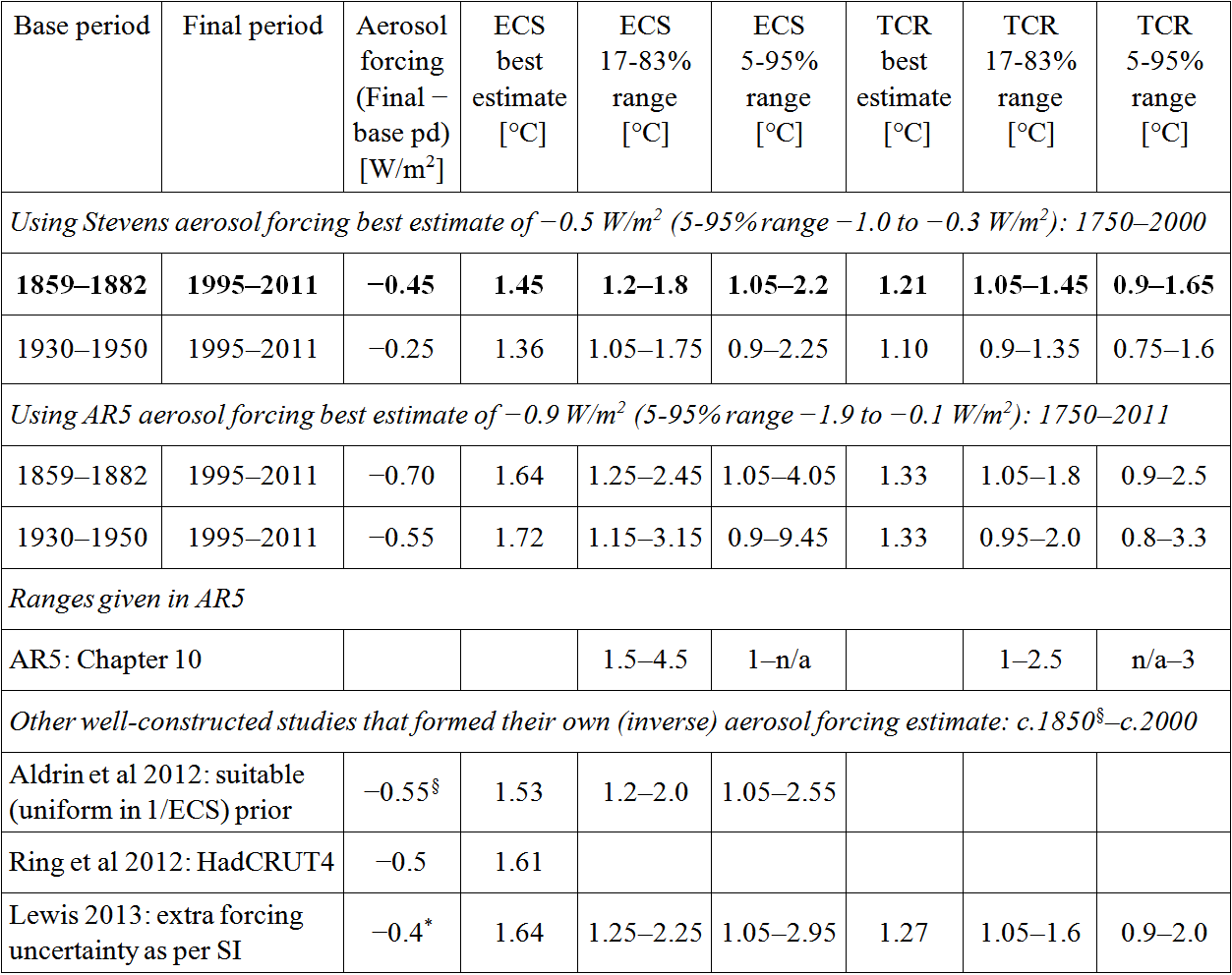
Table 1: Best estimates are medians (50% probability points). Ranges (Ring et al: none given) and aerosol forcings are to the nearest 0.05°C. § Aldrin et al. aerosol forcing estimate is for 1750–2007 and based on replacing the AR4 aerosol forcing distribution used as the prior in the study, which significantly biased the inverse estimate, with the AR5 distribution. * With +0.1 W/m2 added to adjust for omitted black-carbon-on-snow forcing affecting the inverse estimate of aerosol forcing due to its similar fingerprint.
Compared with using the AR5 aerosol forcing estimates, the preferred ECS best estimate using an 1859–1882 base period reduces by 0.2°C to 1.45°C, with the TCR best estimate falling by 0.1°C to 1.21°C. More importantly, the upper 83% ECS bound comes down to 1.8°C and the 95% bound reduces dramatically – from 4.05°C to 2.2°C, below the ECS of all CMIP5 climate models except GISS-E2-R and inmcm4. Similarly, the upper 83% TCR bound falls to 1.45°C and the 95% bound is cut from 2.5°C to 1.65°C. Only a handful of CMIP5 models have TCRs below 1.65°C.
CMIP5 models with high TCRs are able to match the historical instrumental GMST record, or even warm less, mainly because most of them have highly negative aerosol forcing that until recently offset the bulk of greenhouse gas and other positive forcings. The mean aerosol forcing in CMIP5 models for which it has been diagnosed is about −1.2 W/m2 over 1850–2000, two and a half times Stevens’ best estimate.
The new ECS and TCR estimates, and the uncertainty associated with them, can also be presented in the form of probability density functions, as in Figures 1 and 2. The PDFs are skewed due principally to the dominant uncertainty, that in forcing, affecting the denominator of the fractions used to estimate ECS and TCR.
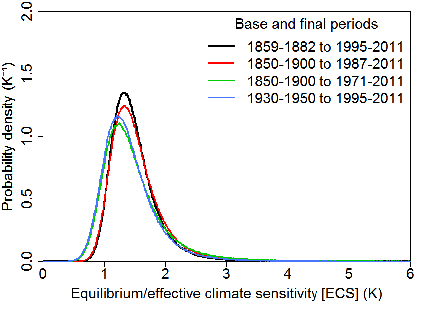 Figure 1: Energy budget estimated PDFs for ECS using Stevens 2015 based aerosol forcing
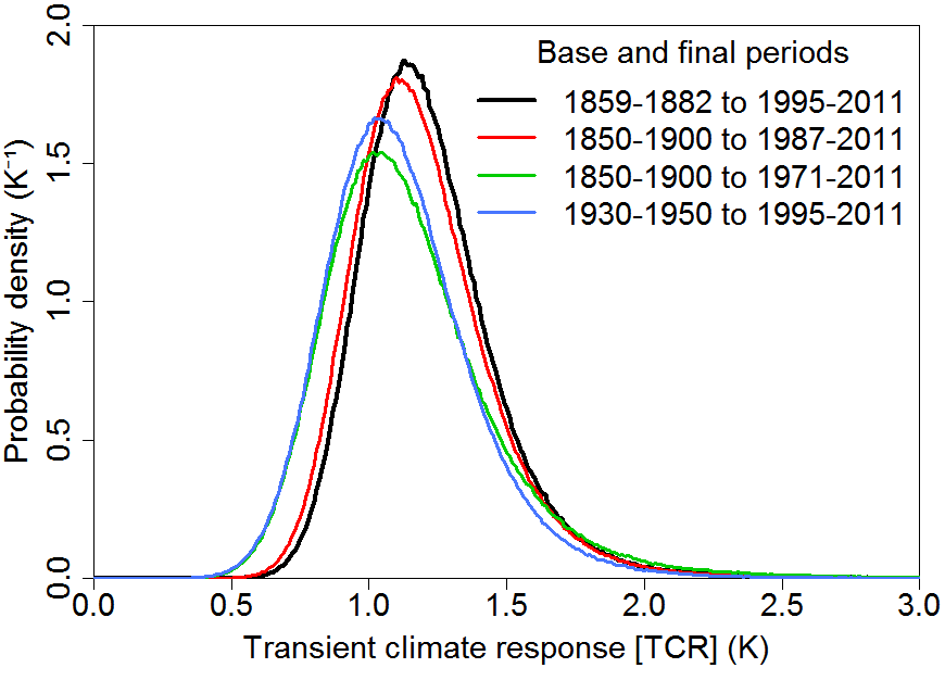 Figure 2: Energy budget estimated PDFs for TCR using Stevens 2015 based aerosol forcing
Appendix: Derivation of a best estimate time series for aerosol forcing from Stevens 2015
The best estimate for direct aerosol forcing (Fari) is taken as −0.15 W/m2 (line 494). The best estimate taken for indirect aerosol forcing (Faci) is that which, when δN/N has a bidirectional factor of two (0.5× to 2.0×) 5–95% uncertainty (line 620; taken as corresponding to a lognormal distribution) and C has a median estimate of 0.1 and a 95% bound of 0.15 (line 584; uncertainty independent and assumed Gaussian), produces a 95% bound for Faci of −0.75 W/m2. That implies a median estimate for Faci of −0.32 W/m2, which when added to the −0.15 W/m2 for Fari gives a best estimate for total aerosol forcing Faer of −0.5 W/m2.
The timeseries for Qa given by Eq.(A9) is used to scale, according to Eq.(1), the best estimate for Faer of −0.5 W/m2 as at 2005 over 1750 to 2011. Values of Qn = 76, α = 0.00167and β = 0.317 are used. Qn is taken from the caption to Fig.2 and α from the last line of Appendix A. The value of β is set to produce a total aerosol forcing of −0.5 W/m2 in 2005. Although giving a slightly different breakdown between Faci and Fari than that just derived, these parameter values result in an almost identical evolution of aerosol forcing.
References
Aldrin M, Holden M, Guttorp P, Skeie RB, Myhre G, Berntsen TK. Bayesian estimation of climate sensitivity based on a simple climate model fitted to observations of hemispheric temperatures and global ocean heat content. Environmetrics 23:253–271 (2012)
Carslaw, K. S., and coauthors. Large contribution of natural aerosols to uncertainty in indirect forcing. Nature, 503 (7474), 67–71 (2013)
Lewis N An objective Bayesian, improved approach for applying optimal fingerprint techniques to estimate climate sensitivity. J Clim 26:7414–7429 (2013)
Lewis N and Curry J A: The implications for climate sensitivity of AR5 forcing and heat uptake estimates, Climate Dynamics doi: 10.1007/s00382-014-2342-y (2014)
Stevens, B. Rethinking the lower bound on aerosol radiative forcing. In press, J.Clim (2015) doi: http://dx.doi.org/10.1175/JCLI-D-14-00656.1


63 Comments
The canonical response will be that relying on Stevens means ignoring….? Would using the IPCC upper bound make much difference? I am not sure if you covered this in your post.
Some of the modelling groups will no doubt be loathe to accept Stevens’ findings. But he is a pretty central figure in the area of cloud processes, which are what largely determine aerosol forcing.
It doesn’t make very much difference if the IPCC AR5 upper bound of −0.1 W/m2 is used instead of −0.3 W/m2 – the ECS and TCR best estimates fall by a few hundredths of a degree, the upper uncertainty bounds by a bit less and the lower uncertainty bounds by a bit more.
What reason will they have for doing so?
it makes their model results look bad.
What reason will they give for doing so?
Nic,
Once again your work drives straight to the heart of AGW theory, thanks for this. You mention that “neither the original Lewis & Curry 2014 ECS and TCR estimates nor the new estimates are significantly influenced by the low increase in surface warming this century.” I recall that you did recalibrate sensitivity estimates with up-to-date temperature data somewhere at some point. Are you planning on further updating your sensitivity estimates using the recent temp data and the new lower bound from Stevens?
Matt
I did extend the estiamtes from 2011 to 2012 in the original Lewis and Curry 2014 paper, and found a negligible impact. I’m not really planning on going beyond 2012, since the AR5 forcing and heat uptake estimates only run to 2011 and adding a longer period than one year becomes more open to argument.
Highly educational as usual. Thanks Nic and Bjorn Stevens. I hope the various modelling groups quickly accept that we have here a more reliable way of estimating aerosol forcing.
As a lukewarmer, central to my comfort with staying between the various extremes of this fight is finding a way to kill the fat tails. Am I correct in saying this paper (if it holds up) does that?
It’s encouraging
Such transience of fat tails;
Been bad to know you.
=============
The only way I can think of killing the fat tail is to hold the forcing and pass the time.
Do low estimates for aerosol cooling imply the 1940-178 drop in global temperatures were not due to coal plant emissions from post-war industrialization?
Yes, they strongly suggest that the main reason for global temperature going down rather than up from 1940 to the mid-1970s despite quite strong greenhouse gas forcing (+0.7 W/m2 for long-lived GHG, +0.85 W/m2 including ozone) lay elsewhere. Internal variability (here the AMO) seems the obvious cause. On Steven’s best estimates, aerosol forcing became a bit under -0.3 W/m2 more negative during this period. Sulphate emissions from coal plants etc. grew rapidly and reached their peak level in the mid/late 1970s.
In the “Dual Critique” of the Stern Review, Carter et al., (2006), we referred to Anderson et al., (2003) ‘Climate forcing by aerosols – a hazy picture’, Science, 300: 1103 – 1104.
We wrote:
More circularity!
Laws, sausage, aerosol forcing delta, and cloud albedo delta…
The PDO/AMO was on its low end of cycle from 1945-1975. According to whom, you ask, why Michael Mann et al (2015). See his Feb post on RealClimate if you can hold your nose through his bragging about creating famous paper and coining the famous term: “Hockey Stick.” Foolish me, I thought Steve was responsible for both.
Correction: Mann was bragging about coining AMO “a term I coined back in 2000, as recounted in my book…” “Hockey Stick” was coined by the late Dr. Jerry Mahlman. Mann’s 2009 email: “Hi Peter, Phil,
No, no, we have to set the record straight! It was Jerry Mahlman who coined the term [“hockey stick”], and in a complimentary (not insulting) way, several years ago.
steve; enough oT for this thread
nic,
I think you could reach a larger audience by
giving the min and max possible values of ECS
and TCR and the meaning of those values so one can
understand the significance of the values in
your tables?
Gerald Browning
Reblogged this on I Didn't Ask To Be a Blog.
There is a workshop on climate sensitivity next week, March 23-27 in Germany. Speakers include Nic Lewis, Lennart Bengtsson, James Annan and Bjorn Stevens. (HT @ed_hawkins).
The title of Stevens’s talk is
“Some (not yet entirely convincing) reasons why 2.0 < ECS < 3.5"
which suggests he does not agree with Nic's argument.
Paul Matthews, thanks for posting that. Sounds like a lot of fascinating discussion will take place. I wonder if there have been previous workshops on the topic, or if it’s only “hot” now.
Nic, it would be great if, after the workshop, you could post a summary of how Stevens arrives at his ECS range. Or convince him to make a post somewhere. Apparently his approach differs from that of Lewis & Curry 2014.
It would be wonderful to have a summary of the entire workshop. Perhaps James Annan and Tamsin Edwards would consider it for their blogs. I suspect that this would be more informative than the entire AR5 discussion of the topic.
Paul:
In light of the caveat, might he be trying to make it easier for the current generation of modellers to take his methods on board?
Nic, thanks for this. The deus ex machina nature of historical aerosols has always been frustrating, so nice to see some light shed on this,
That’s a bingo. Me too.
Nic wrote:
Nic, there are frustrating issues with the SST record around 1940 regarding bucket adjustments. I discussed this in some early CA posts e.g.
In a post in 2007 https://climateaudit.org/2007/12/23/rasmus-the-chevalier-and-bucket-adjustments/, I noted that the SST history used in Woodruff and Paltridge 1981 had a very different appearance through 1960 than the Folland’s subsequent bucket-adjusted SST data that appears to have been tailored to reconcile to Phil Jones’ land data. In statistical terms, there is one or more degree of freedom in the adjustments that isn’t obvious in the published HadCRU data.
In another 2007 post https://climateaudit.org/2007/03/18/the-team-and-pearl-harbor/, I observed that gradual changeover from buckets to inlets would eliminate the 1960s hiatus.
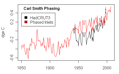
The ICOADS data is vast and interesting. In a quick review, the following graphic from a past post still looks very compelling to me as showing the value of mixed effects statistical analysis on SST data. In this case, changes in SST provenance look very much responsible for the 1940s blip in SST values.
At the time, I observed that it seemed possible that the 20th century temperature increase might be uniform than posited in the HadCRU data.
Steve,
Thanks; interesting.
Steve, if the SST blip is a product of a measuring/computational error, what then explains the “blip” in the land data?
Are we to assume that the ocean actually warmed by 0.2 K or so cca 1945-1975 while the land cooled by 0.6 K in the same period (at least according to the NAS data from 1975)?
There are several other confounding factors for SST during the 1939-45 period.
1. Ship routing changed extensively. The sampling pattern must have been vastly different than before or after the war.
2. Most shipping travelled in convoys. Allied convoys typically consisted of columns of about 5 ships, which means that 80% of samples are not from undisturbed surface water, but from water thad had been churned up by at least one other ship.
3. Huge amounts of oil were released into the ocean, particularly along shipping routes. Contemporary accounts often mention oil spills and oil films. How did this affect sea roughness and evaporation?
that still does not explain the land blip.
” In statistical terms, there is one or more degree of freedom in the adjustments that isn’t obvious in the published HadCRU data.”
yup.
Seems a major hassle of climate science is the lack of good quality measurements to work with. I mean, even satellite-based radiometers can be interpreted in different ways that lead to different trends (uah vs rss).
The alleged measurement diversity (and subsequent adjustments) in HadSST3 are particularly troubling to those of us who believe sea surface temperature (and HadSST3) is the most accurate indicator of climate, and very bad news for any models which seek to reproduce it.
Nic, Excellent post, as usual. One additional comment: I also have employed a relatively simple two-hemisphere energy-balance model to derive an inverse aerosol forcing “best fit” over the complete period 1850 to 2014. I obtain sensitivity numbers very close to yours and median aerosol forcings close to Stevens’ values. If, in addition, I also allow for the possible influence of natural internal variability driven, for example, by the PDO and AMO, the “best fit” median ECS reduces to 1.2 to 1.3 degrees C, with net aerosol forcing changes between 1850 and 2014 (including the effects of black carbon and black carbon on snow) near zero. In both cases predicted temperatures are close to the HadCRUT4 observations in the 1990 to 2014 time period; that is, there is little “pause” to explain – implying that the CMIP5 GCM “pause” problem is most likely an artifact of too-high sensitivity. Projections to 2100 considering natural variability and using RCP45 forcing yields temperature increases from 1850 to 2100 of less than 1.4 degrees C – well below the arbitrary IPCC 2 degree C “dangerous” level. In this case even the (IMHO unrealistic) rcp85 forcing yields 2100 temperature increases of only a little over 2 degrees C. Attempts by the “climate science” community to dismiss the sensitivity issue as unimportant seem misplaced.
Keith Jackson
Keith, Thanks for sharing your findings. I agree that the ‘pause’ seems unsurprising given the influence of internal variability and the rapid warming experienced over the previous 25 years.
Thank you Nic, I highly enjoyed both reading this and tracing back through to your original report. In fact as I literally never post here (mainly because of a lack of substantial climate knowledge), this place has served as a beacon to me in education, so in turn I appreciate all of the contributors and many of the comments as well (though, I suppose that also is contribution). Although I will say if anyone needs help with programming or such I’d be happy to help them, as my math and programming skills are up to par perhaps even a couple birdies to make it better than par occasionally. I did want to at least post a comment somewhere, and being as I enjoyed this post, here is as good as anywhere, to thank everyone here. Keep posting when you guys each put out new books and publications, I buy em all. 🙂
Nic, thanks again for an informative post on an area of climate science that I think cuts right to the critical matters of AGW and the best available method of comparing model temperature output to the observed. Separating the deterministic part of temperature series from the internal variability (noise) is what is of critical importance with regards to AGW, since we have little to no control over the chaotic noise.
I continue to work on analytically finding the best fitting deterministic trends in modeled and observed temperature series and in turn obtaining some theoretical support for this method by the correlation of SSA derived trends of model temperature series to model TCR values. I can reach correlation levels in excess of 0.8 with the data scattered rather evenly about a regression line. I can show that the SSA trends include very little noise by comparing the variance of SSA trends of multiple runs of individual models with the variation in SSA trends between individual models. I also judge that the only sufficiently large variation outside GHG levels – and its effects on individual models as expressed by TCR – keeping the regression residuals this large are the differing aerosol effects from individual models. Unfortunately I have not been able to find a decent proxy for the aerosol effects to include in a multiple regression. I do plan to look closer at the various model RCP scenarios and the various prescribed and varying levels of GHGs and aerosols.
By the way, Nic, I was curious about the potential effects of auto correlation of the residuals of the M&F regression and the effect that would have on the confidence intervals (and need for adjustment) for the regression variable coefficients. I received the input data for the regression from Jochem Marotzke, but have not had time to look at it yet.
Hermann,
All the factors that can affect climate need to be fully characterized, it cannot be done by intuition. Nic is on as good a track as anybody and way better than most. If you want to find out more about albedo you cannot do better than this recent paper:
Nic, nice work again. Do you mostly agree with Mann’s recent chart on PDO/AMO which, if Mann accepts, seems to call for an IPCC attribution correction? The reasoning (if not clear) is that since the late 1990s temp rise was due in large degree to a convergent peak of PDO/AMO then then the IPCC’s attribution of temp rise being largely AGW needs to be revised. Also, as Mann’s chart shows PDO/AMO in downcycle for another 10-15 years this seems to be inoculating against anticipated criticism from a lasting pause. But at the same time wouldn’t it need to be adopted into the numbers and thus lower ECS in models? And, while they are doing that they can fix the aerosols. So I am sure they are thanking you and Stevens for the convenient timing.
I meant lowering ECS in addition to the amount your’s and Steven’s work would imply.
Nic,
The numbers in your tables are clearly derived from some numbers in each of the two chosen time periods. Please provide the mathematical formula used to derive the numbers in the tables and describe the variables used from each of the time periods so that one can check the assumptions that have been made. You gloss over the definitions of ECS and TCR and those definitions are crucial to your arguments. Clearly your arguments can be presented in this more clear and complete way so that nonspecialists can understand them and check them.
Jerry
Thanks Nic,
Interesting stuff on Stevens paper. Sadly pay-walled , so hard to assess properly.
I find your article a little hard to follow since in several places you refer to simply “aerosol forcing” rather than direct indirect, total or effective aerosol forcing . This leaves the reader to parse the context, apply and understanding of the physics / modelling involved and then infer what you were referring to.
This makes it rather imprecise and hard to follow and difficult to get point being made.
“CMIP5 models with high TCRs are able to match the historical instrumental GMST record, or even warm less, mainly because most of them have highly negative aerosol forcing that until recently offset the bulk of greenhouse gas and other positive forcings. The mean aerosol forcing in CMIP5 models for which it has been diagnosed is about −1.2 W/m2 over 1850–2000”
Here I would guess from the presence of the word “diagnosed” that you are referring to “effective” since the direct forcing is a programmed-in parameter.
Now it is very likely that both “effective”aerosol forcing and “effective” AGW forcing have been over estimated and played off against each other as you say. This relates to misdiagnosis of cloud and other feedbacks.
If the direct aerosol forcing is also made low then feedbacks stay about the same and we are stuck with more sensitive climate which seems to be where Stevens is to judge by the title of his discussion next week.
I cannot follow this aspect w.r.t. Stevens paper since I don’t have it but the level of direct forcing is just as important to the overall discussion and I don’t see how that can be satisfactorily estimated from the available data.
My Pinatubo article [ http://judithcurry.com/2015/02/06/on-determination-of-tropical-feedbacks/ ] suggests a much stronger direct aerosol forcing from volcanoes than is *currently* used in models and this is based on fairly detailed energy budget and SST data. The reason direct forcing was dropped was parameter juggling to reconcile model output whilst maintaining high sensitivity ( ie positive cloud feedbacks ).
The other way to go is to return to earlier higher values of direct forcing which implies more negative feedbacks. This argues against indirect effects which act in the same sense, ie positive elements of “net positive” feedback.
The link to lower stratospheric temperature still suggests that El Chichon and Mt P had a lasting warming effect on surface temps, beyond the initial disturbance. This may include flushing out low levels of industrial pollution that had been building up post 1960 expansion.
Simply playing off aerosols ( natural or industrial ) vs GHG forcing is not enough and care is needed not to fall into the trap of assuming all else is correct. It isn’t.
Greg Goodman
Wispy winds wander,
Wonder over and under,
Cloud climate models.
===========
By aerosol forcing I meant total aerosol forcing, direct plot indirect. This is stated in the Appendix, and I say earlier that “Stevens derives a lower limit for total aerosol forcing, from 1750 to recent years, of −1.0 W/m2”.
Since indirect aerosol forcing reflects the effects of aerosol on clouds, total aerosol forcing should be regarded as an effective radiative forcing (ERF).
Greg Goodman: “Sadly pay-walled…”
I saw this link elsewhere.
thanks 😉
Stevens:
Since CO2 forcing is also logarithmic, I don’t follow this idea.
Looking at Stevens’ figure 1, it shows biggest rate of increase in emissions from 1950 to 1970; from then on nearly flat with a slight dip in 1990.
Now looking at model ‘tas’ (near surface air temp) deviations from hadCRUT4 surface temp:
The big dip ( models fail to match warming dT/dt ) centred on 1960 could be partly explained by too much effective aerosol forcing, particularly for high TCR group.
However, the largest peak deviation in both groups is centred on 1970 and is about equal for both, and shows much stronger warming in models than was actually happening.
It is hard to relate that to the constant high level of emissions, if they are weighted too strongly.
That is not to say that Stevens is incorrect but it does not seem to be the cause of the major deviations in the 20th c. record. Though it may be a contributory factor.
OTOH, 1970 was a weak solar cycle and 1960 a very strong one. Those major deviations seem to suggest incorrect modelling of solar effects.
Greg, I agree that we’re not ready yet to attempt to analyze the change in industrial emitted aerosols in relation to emitted GHG due to the lack of consensus on PDO/AMO and other temperature record interfering effects. But, once certainty increases sufficiently in some of these areas, including aerosols, the matrix becomes easier to solve for the others. Progress accelerates.
On a different not, if aerosols truly are less effective than thought we have finally put to rest the issue that created consensus for a strong aerosol effect, the 1970-73 alarm that that pollution would pre-maturely end our balmy inter-glacial tipping us to fall in ice age spiral. I remember the warning was even in my 4th grade Weekly Reader.
I don’t pretend to be a scientist. My experience with climate is totally subjective, but I KNOW, beyond the shadow of doubt, that this argument includes smoke and mirrors, from both sides. What is happening is that we are arguing over change from the status quo, that is necessary, regardless of AGW veracity or not. What we are doing to our physical environment is NOT sustainable. All we are doing is finding excuses for not doing the intelligent thing, which is getting off of fossil fuels completely, and cleaning up our act as soon as possible. There is no long term benefit to the planet for continuing this argument, which only slows down the necessary change. Is it important to study it? Of course, because it is important to more fully understand the implication of events, not just for predictive purposes but for mitigation purposes. We just need to detach from the politics and political ambitions of a few and ACT.
Steve: Stephen Leacock described the policy of “just ACT” as follows: “Lord Ronald said nothing; he flung himself from the room, flung himself upon his horse and rode madly off in all directions”. “Gertrude the Governess”, Nonsense Novels (1911).
It is blog editorial policy that commenters comment on the post rather than trying to argue the pros and cons of everything in the world, as otherwise comments on all threads quickly become identical.
snip – no need to rise to this
Ah, forgot Lord Ronald, activist supreme.
My God: Haven’t heard this since a teacher read it to us in the tenth grade. Thanks!
phil
the phrase has stuck in my mind since high school as well. I think that it aptly characterizes the sort of policy that Michael Kelly criticizes and opposes.
Michael Kelly’s pretty much the most thoughtful and articulate critic we have.
Thanks for this most educational post (and comments) . Three cheers for real (unbiased) science! The 95% meme nauseates me.
Quite funny. On aTTP site everybody was paging Karsten. The man appeared, skimmed the paper quickly after a pub session, said he did not like it too much, found it needs to be debunked and said that he’ll see what he can do about it. And aTTP was happy.
Because you refused to clarify the definitions of ECS and TCR, I went to your manuscript with Curry. You have more parameters to adjust than a climate model. And then you use info from AR5 that is questionable to begin witn. An energy balance model is also suspect.
I like your results, but have no confidence in them based on these issues and your refusal to clarify your approach. Now I know why that is the case.
Jerry
From, per Gavin, deep philosophical differences, to, per me, deep paleontological sophistries, playing now at the Ringberg Auditorium.
=================
Clearly it’s “compelling” to you because it says what you want to believe.
The Empire strikes back:
Click to access AerosolForcing-Statement-BjornStevens.pdf
Funny, they don’t usually correct “misinterpretations” when the press exaggerates the implications of their work. Why would they choose to do so in this case? 😉
Amazing. In what other field of science would you have such pledges of allegiance? This really is reminiscent of the Soviet Union in the Stalin era.
It surely be interesting to see how history will look back on this. Currently Neil Degrasse Tyson’s “Cosmos” compares Hansen to Galileo.
sounds like he was taken hostage and asked to sign this ransom letter. Do you think he wrote it?
Good analysis. I have difficulty accepting the aerosol “negative forcing” idea because “aerosols” don’t seem to be a correction to satellite temperature measurements in the IR to ground based temperature measurements. I can’t see how aerosol reflectivity would not influence satellite measurements, be evidently variable
24 Trackbacks
[…] Audit hva som er konsekvensene for ECS/TCS estimatene og han har satt opp en fin tabell for dette her. Hovedpunktet er som følger: Compared with using the AR5 aerosol forcing estimates, the preferred […]
[…] at Climate Audit, Nic Lewis reports on the publication of a very important paper in Journal of […]
[…] all excited, because it has implication for climate sensitivity. Nic Lewis has a post on Climate Audit and on Climate Etc.. It’s also mentioned on Bishop-Hill and, I presume (although I […]
[…] Lewis reports on the publication of a very important paper in Journal of Climate. Bjorn Stevens has created a new […]
[…] […]
[…] Curry and Steve McIntyre hosted a guest post by Nic Lewis on a recent paper by Bjorn Stevens. The paper essentially reports […]
[…] https://climateaudit.org/2015/03/19/the-implications-for-climate-sensitivity-of-bjorn-stevens-new-aer… […]
[…] new scientific paper has driven yet another nail into the coffin of Catastrophic Anthropogenic Global Warming theory. […]
[…] Qui, se volete approfondire un po’. […]
[…] was quick to realize the implications of the Stevens’ results. In a blog post over at Climate Audit, Lewis takes us through his calculations as to what the new aerosols cooling estimates mean for […]
[…] https://climateaudit.org/2015/03/19/t…forcing-paper/ 3 Add Dyzalot to Rail […]
[…] revised his findings based on the Max Planck aerosol study and found something astounding: climate sensitivity drops […]
[…] revised his findings based on the Max Planck aerosol study and found something astounding: climate sensitivity drops […]
[…] revised his findings based on the Max Planck aerosol study and found something astounding: climate sensitivity drops […]
[…] revised his findings based on the Max Planck aerosol study and found something astounding: climate sensitivity drops […]
[…] revised his findings based on the Max Planck aerosol study and found something astounding: climate sensitivity drops […]
[…] revised his findings based on the Max Planck aerosol study and found something astounding: climate sensitivity drops […]
[…] to the blog Climate Audit, climate researcher Nic Lewis found Stevens’ study blew a hole through global warming and climate change study and even a recent […]
[…] The lower bound is lower? Hmmm…. This study has significant implications as discussed here. […]
[…] […]
[…] 19, 2015, Nic Lewis explained the paper’s far-reaching implications at Steve McIntyre’s Climate Audit and Judith Curry’s Climate Etc.: Also the climate sensitivity gets further limited, and most […]
[…] on aerosol radiative forcing” has led to some confusion. The article states, referring to a blog post of mine at Climate Audit, “The misinterpretation of Stevens’ paper began with Nic […]
[…] Professor Bjorn Stevens publicerade en artikel för några veckor sedan som vållade ett visst rabalder bland klimatforskarna eftersom artikelns resultat implicerar att uppskattningen av den s.k. klimatkänslighetens övre intervall måste minska. (I klartext skulle ju detta resultat innebära att klimathotet är en överdrift.) Se exempelvis Nicholas Lewis tolkning här. […]
[…] called “climate sensitivity” was 1.64 degrees Celsius.What do you think? Lewis revised his findings based on the Max Planck aerosol study and found something astounding: climate sensitivity drops […]