A guest article by Nic Lewis
Introduction
In April 2014 I published a guest article about statistical methods applicable to radiocarbon dating, which criticised existing Bayesian approaches to the problem. A standard – subjective Bayesian – method of inference about the true calendar age of a single artefact from a radiocarbon date determination (measurement) involved using a uniform-in-calendar-age prior. I argued that this did not, as claimed, equate to not including anything but the radiocarbon dating information, and was not a scientifically sound method for inference about isolated examples of artefacts.[1]
My article attracted many comments, not all agreeing with my arguments. This article follows up and expands on points in my original article, and discusses objections raised.
First, a brief recap. Radiocarbon dating involves determining the radiocarbon age of (a sample from) an artefact and then converting that determination to an estimate of the true calendar age t, using a highly nonlinear calibration curve. It is this nonlinearity that causes the difficulties I focussed on. Both the radiocarbon determination and the calibration curve are uncertain, but errors in them are random and in practice can be combined. A calibration program is used to derive estimated calendar age probability density functions (PDFs) and uncertainty ranges from a radiocarbon determination.
The standard calibration program OxCal that I concentrated on uses a subjective Bayesian method with a prior that is uniform over the entire calibration period, where a single artefact is involved. Calendar age uncertainty ranges for an artefact whose radiocarbon age is determined (subject to measurement error) can be derived from the resulting posterior PDFs. They can be constructed either from one-sided credible intervals (finding the values at which the cumulative distribution function (CDF) – the integral of the PDF – reaches the two uncertainty bound probabilities), or from highest probability density (HPD) regions containing the total probability in the uncertainty range.
In the subjective Bayesian paradigm, probability represents a purely personal degree of belief. That belief should reflect existing knowledge, updated by new observational data. However, even if that body of knowledge is common to two people, their probability evaluations are not required to agree,[2] and may for neither of them properly reflect the knowledge on which they are based. I do not regard this as a satisfactory paradigm for scientific inference.
I advocated taking instead an objective Bayesian approach, based on using a computed “noninformative prior” rather than a uniform prior. I used as my criterion for judging the two methods how well they performed upon repeated use, hypothetical or real, in relation to single artefacts. In other words, when estimating the value of a fixed but unknown parameter and giving uncertainty ranges for its value, how accurately would the actual proportions of cases in which the true value lies within each given range correspond to the indicated proportion of cases? That is to say, how good is the “probability matching” (frequentist coverage) of the method. I also examined use of the non-Bayesian signed root log-likelihood ratio (SRLR) method, judging it by the same criterion.
Bayesian parameter inference
A quick recap on Bayesian parameter inference in the continuously-valued case, which is my exclusive concern here. In the context we have here, with a datum – the measured C14 age (radiocarbon determination) dC14 – and a parameter t, Bayes’ theorem states:
p(t|dC14) = p(dC14|t) p(t) / p(dC14) (1)
where p(x|y) denotes the conditional probability density for variable x given the value of variable y. Since p(dC14) is not a function of t, it can be (and usually is) replaced by a normalisation factor set so that the posterior PDF p(t|dC14) integrates to unit probability. The probability density of the datum taken at the measured value, expressed as a function of the parameter (the true calendar age t), p(dC14|t), is called the likelihood function. The construction and interpretation of the prior distribution or prior, p(t), is the critical practical difference between subjective and objective Bayesian approaches. In a subjective approach, the prior represents as a probability distribution the investigator’s existing degree of belief regarding varying putative values for the parameter being estimated. There is no formal requirement for the choice of prior to be evidence-based, although in scientific inference one might hope that it often would be. In an objective approach, the prior is instead normally selected to be noninformative, in the sense of letting inference for the parameter(s) of interest be determined, to the maximum extent possible, solely by the data.
A noninformative prior primarily reflects (at least in straightforward cases) how informative, at differing values of the parameter of interest, the data are expected to be about that parameter. In the univariate parameter continuous case, Jeffreys’ prior is known to be the best noninformative prior, in the sense that, asymptotically, Bayesian posterior distributions generated using it provide closer probability matching than those resulting from any other prior.[3] Jeffreys’ prior is the square root of the (expected) Fisher information. Fisher information – the expected value of the negative second derivative of the log-likelihood function with respect to the parameters, in regular cases – is a measure of the amount of information that the data, on average, carries about the parameter values. In simple univariate cases involving a fixed, symmetrical measurement error distribution, Jeffreys’ prior will generally be proportional to the derivative of the data variable being measured with respect to the parameter.
To simplify matters, I worked with a stylised calibration curve, which conveyed key features of the nonlinear structure of the real calibration curve – alternating regions where the radiocarbon date varied rapidly and very slowly with calendar age – whilst retaining strict monotonicity and having a simple analytical derivative. Figure 1, a version of Figure 2 in the original article, shows the stylised calibration curve (black) along with the error distribution density for an example radiocarbon date determination (orange). The grey wings of the black curve represent a fixed calibration curve error, which I absorb into the C14 determination error, assumed here to have a Gaussian distribution with fixed, known, standard deviation. The solid pink line shows the Bayesian posterior probability density function (PDF) using a uniform in calendar age prior. The dotted green line shows the noninformative Jeffreys’ prior used in the objective Bayesian method, which reflects the derivative of the calibration curve. The posterior PDF using Jeffreys’ prior is shown as the solid green line. The dashed pink and green lines, added in this version, show the corresponding posterior CDF in each case.
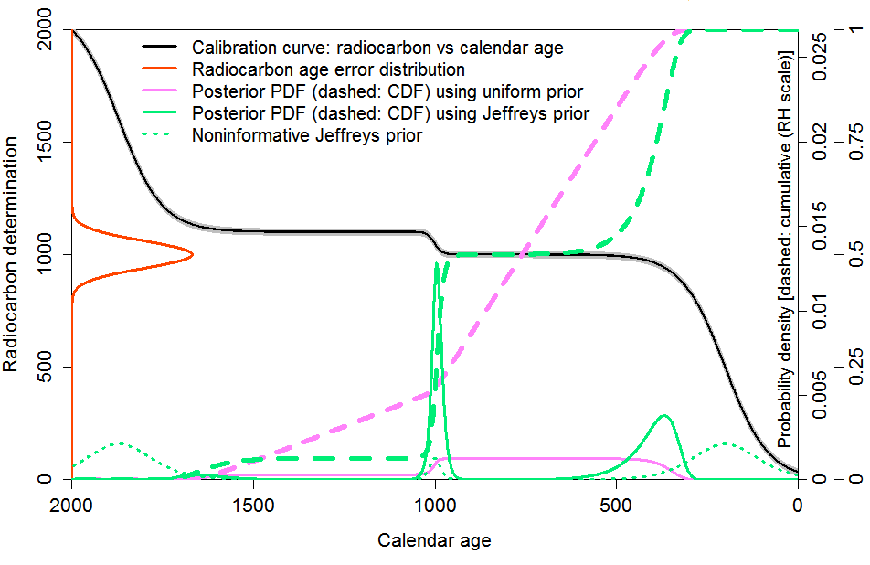 Fig. 1: Bayesian inference using uniform and objective priors with a stylised calibration curve and
an example observation; combined measurement/calibration error standard deviation 60 RC years.
The shape of the objective Bayesian posterior PDF
The key conclusions of my original article were:
“The results of the testing are pretty clear. In whatever range the true calendar age of the sample lies, both the objective Bayesian method using a noninformative Jeffreys’ prior and the non-Bayesian SRLR method provide excellent probability matching – almost perfect frequentist coverage. Both variants of the subjective Bayesian method using a uniform prior are unreliable. The HPD regions that OxCal provides give less poor coverage than two-sided credible intervals derived from percentage points of the uniform prior posterior CDF, but at the expense of not giving any information as to how the missing probability is divided between the regions above and below the HPD region. For both variants of the uniform prior subjective Bayesian method, probability matching is nothing like exact except in the unrealistic case where the sample is drawn equally from the entire calibration range”
For many scientific and other users of statistical data, I think that would clinch the case in favour of using the objective Bayesian or the SRLR methods, rather than the subjective Bayesian method with a uniform prior. Primary results are generally given by way of an uncertainty range with specified probability percentages, not in the form of a PDF. Many subjective Bayesians appear unconcerned whether Bayesian credible intervals provided as uncertainty ranges even approximately constitute confidence intervals. Since under their interpretation probability merely represents a degree of belief and is particular to each individual, perhaps that is unsurprising. But, in science, users normally expect such ranges to be at least approximately valid as confidence intervals, so that, upon repeated applications of the method – not necessarily to the same parameter – in the long run the true value of the parameter being estimated would lie within the stated intervals in the claimed percentages of cases.
However, there was quite a lot of pushback against the rather peculiar shape of the objective Bayesian posterior PDF resulting from use of Jeffreys’ prior. It put near zero probability on regions where the data, although being compatible with the parameter value, was insensitive to it. That is, regions where the data likelihood was significant but the radiocarbon determination varied little with calendar age, due to the flatness of the calibration curve. The pink, subjective Bayesian posterior PDF was generally thought by such critics to be more realistically-shaped. Underlying that view, critics typically thought that there was relevant prior information about the age distribution of artefacts that should be incorporated, by reflecting through use of a uniform prior a belief that an artefact was equally likely to come from any (equal-length) calendar age range. Whether or not that is so, the uniform prior had instead been chosen on that basis that it did not introduce anything but the RC dating information, and I argued against it on that basis.
I think the view that one should reject an objective Bayesian approach just on the basis that the posterior PDF is gives rise to is odd-looking is mistaken. In most cases, what is of concern when estimating a fixed but uncertain parameter, here calendar age, is how well one can reliably constrain its value within one or more uncertainty ranges. In this connection, it should be noted that although the Jeffreys’ prior will assign low PDF values in a range where likelihood is substantial but the data variable is insensitive to the parameter value, the uncertainty ranges that the resulting PDF gives rise to will normally include that range.
Probability matching
I think it is best to work with one-sided ranges, which unlike two-sided ranges are uniquely defined, whereas an 80% (say) range could be 5–85% or 10–90%. A one-sided x% range is the range from the lowest possible value of the parameter (here, zero) to the value, y, at which the range contains x% of the posterior probability. An x1–x2% range or interval for the parameter is then y1 − y2, where y1 and y2 are the (tops of the) one-sided x1% and x2% ranges. An x% one-sided credible interval derived from a posterior CDF relates to Bayesian posterior probability. By contrast, a (frequentist) x% one-sided confidence interval bounded above by y is calculated so that, upon indefinitely repeated random sampling from the data uncertainty distribution(s) involved, the true parameter value will lie below the resulting y in x% of cases (i.e., with a probability of x%).
By definition, an accurate confidence interval bound exhibits exact probability matching. If one-sided Bayesian credible intervals derived using a particular prior pass the matching test for all values of x then they and the prior used are said to be probability matching. From a scientific viewpoint, probability matching is highly desirable. It implies – if the statistical analyses have been performed (and error distributions assessed) correctly – that, for example, only in one study out of twenty will the true parameter value lie above the reported 95% uncertainty bound. In general, Bayesian posteriors can only, at best, be approximately probability matching. But the simple situation presented here falls within the “location parameter” exception to the no-exact-probability-matching rule, and use of Jeffreys’ prior should in principle lead to Bayesian one-sided credible intervals exhibiting exact probability matching.
The two posterior PDFs in Figure 1 imply very different calendar age uncertainty ranges. However, as I showed in the original article, if a large number of true calendar ages are sampled in accordance with the assumed uniform distribution over the entire calibration curve (save, to minimise end-effects from likelihood lying outside the calibration range, 100 years at each end), and a radiocarbon date determined for each of them in accordance with the calibration curve and error distribution, then both methods provide excellent probability matching. This is to be expected, but for different reasons in the subjective and objective Bayesian cases.
Figure 2, a reproduction of Figure 3 in the original article, shows the near perfect probability matching in this case for both methods. At all one-sided credible/confidence interval sizes (upper level in percent), the true calendar age lay below the calculated limit in almost that percentage of cases. As well as results for one-sided intervals using the subjective Bayesian method with a uniform prior and the objective Bayesian method with Jeffreys’ prior, Figure 2 shows comparative results on two other bases. The blue line is for two-sided HPD regions, using the subjective Bayesian method with a uniform prior. An x% HPD region is the shortest interval containing x% of the posterior probability and in general does not contain an equal amount of probability above and below the 50% point (median). The dashed green line uses the non-Bayesian signed root log-likelihood ratio (SRLR) method, which produces confidence intervals that are in general only approximate but are exact when a normal distribution or a transformation thereof is involved, as here.
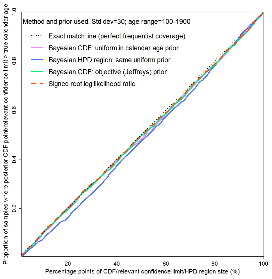 Fig. 2: Probability matching: repeated draws of parameter values; one C14 measurement for each
Figure 2 supports use of a subjective Bayesian method in a scenario where there is an exactly known prior probability distribution for the unknown variable of interest (here, calendar age), many draws are made at random from it and only probability matching averaged across all draws is of concern. The excellent probability matching for the subjective Bayesian method shows that stated uncertainty bounds using it are valid when aggregated over samples of parameter values drawn randomly, pro rata to their known probability of occurring. In such a case, Bayes’ theorem follows from the theory of conditional probability, which is part of probability theory as rigorously developed by Kolmogorov.[4]
However, the problem of scientific parameter inference is normally different. The value of a parameter is not drawn from a known probability distribution, and does not vary randomly from one occasion to another. It has a fixed, albeit unknown, value, which is the target of inference. The situation is unlike the scenario where the distribution from which parameter values are drawn is fixed but the parameter value varies between draws, and, often, no one drawn parameter value is of particular significance (a “gambling scenario”). Uncertainty bounds that are sound only when parameter values are drawn from a known probability distribution, and apply only upon averaging across such draws, are not normally appropriate for scientific parameter inference. What is wanted are uncertainty bounds that are valid on average when the method is applied in cases where there is only one, fixed, parameter value, and it has not been drawn at random from a known probability distribution.
In Figure 2, values for the unknown variable are drawn many times at random from a specified distribution and in each instance a single subject-to-error observation is made. The testing method corresponds to a gambling scenario: it is only the average probability matching over all the parameter values drawn that matters. Contrariwise, Figure 3 corresponds to the parameter inference case, where probability matching at each possible parameter value separately matters. I selected ten possible parameter values (calendar ages), to illustrate how reliable inference would typically be when only a single, fixed, parameter value is concerned. I actually drew the parameter values at random, uniformly, from the same age range as in Figure 2, but I could equally well have chosen them in some other way. For each of these ten values, I drew 5,000 radiocarbon date determinations randomly from the measurement error distribution, rather than a single draw as used for Figure 2, and computed one-sided 1% to 100% uncertainty intervals. Each of the lines corresponds to one of the ten selected parameter values.
As can be seen, the objective Bayesian and the SRLR methods again provide almost perfect probability matching in the case of each of the ten parameter values separately (the differences from exact matching are largely due to end effects). But probability matching for the subjective Bayesian method using a uniform prior was poor – awful over much of the probability range in most of the ten cases. Whilst HPD region coverage appears slightly less bad than for one-sided intervals, only the total probability included in the HPD region is being tested in this case: the probabilities of the parameter value lying above the HPD region and lying below it may be very different from each other. Therefore, HPD regions are useless if one wants the risks of over- and under-estimating the parameter value to be similar, or if one is primarily concerned about one or other of those risks.
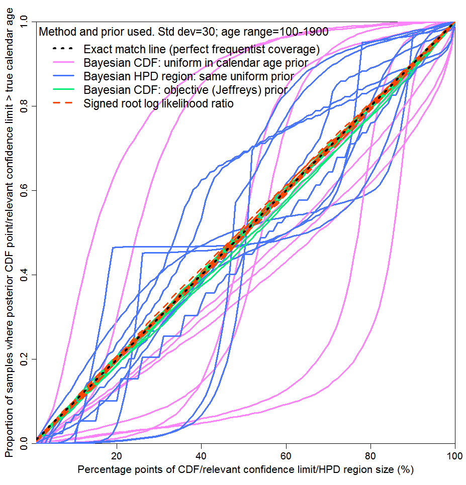
Fig. 3: Probability matching for each of 10 artefacts with ages drawn
from a uniform distribution: 5000 C14 measurements for each
I submit that Figure 3 strongly supports my thesis that a uniform prior over the calibration range should not be used here for scientific inference about the true calendar age of a single artefact, notwithstanding that it gives rise to a much more intuitively-appealing posterior PDF than use of Jeffreys’ prior. It may appear much more reasonable to assume such a uniform prior distribution than the highly non-uniform Jeffreys’ prior. However, the wide uniform distribution does not convey any genuine information. Rather, it just causes the posterior PDF, whilst looking more plausible, to generate misleading inference about the parameter.
What if an investigator is only concerned with the accuracy of uncertainty bounds averaged across all draws, and the artefacts are known to be exactly uniformly distributed? In that case, is there any advantage in using the subjective Bayesian method rather than the objective one, apart from the posterior PDFs looking more acceptable? Although both methods deliver essentially perfect probability matching, one might generate uncertainty intervals that are, on average, smaller than those from the other method, in which case it would arguably be superior. Re-running the Figure 2 case did indeed reveal a difference. The average 5–95% uncertainty interval was 736 years using the objective Bayesian method. It was rather longer, at 778 years, using the subjective Bayesian method.
So in this case the objective Bayesian method not only provides accurate probability matching for each possible parameter value, but on average it generates narrower uncertainty ranges even in the one case where the subjective method also provides probability matching. Even the less useful HPD 90% regions, which say nothing about the relative chances of the parameter value lying below or above the region, were on average only slightly narrower, at 724 years, than the objective Bayesian 5–95% regions. The failure of the subjective Bayesian method to provide narrower 5–95% uncertainty ranges reflects the fact that knowing the parameter is drawn randomly from a wide uniform distribution provides negligible useful information about its value.
Is standard usage of Bayes’ theorem appropriate for parameter inference?
My tentative interpretation of the difference between inference using a uniform prior in Figures 2 and 3 is this. In the Figure 2 case, the calendar age is a random variable, in the Kolmogorov sense (a KRG). Each trial involves drawing an artefact, and for it an associated RC determination, at random. There is a joint probability function involved and a known unconditional probability distribution for calendar age. The conditional probability density of calendar age for an artefact given its RC determination is then well defined, and given by Bayes’ theorem. But in the Figure 3 case, taking any one of the ten selected calendar ages on their own, there is no joint probability distribution involved. The parameter (calendar age) is not a KRG;[5] its value is fixed, albeit unknown. A conditional probability density for the calendar age of the artefact is therefore not validly given, by Bayes’ theorem, as the product of its unconditional density and the conditional density of the RC determination, since the former does not exist.[6]
Under the subjective Bayesian interpretation, the standard use of Bayes’ theorem is always applicable for inference about a continuously-valued fixed but unknown parameter In my view, Bayes’ theorem may validly be applied in the standard way in a gambling scenario but not, in general, in the case of scientific inference about a continuously-valued fixed parameter – although it will provide valid inference in some cases and lead only to minor error in many others. The fact that the standard subjective uses of Bayes’ theorem should never lead to internal inconsistencies in personal belief systems does not mean that they are objectively satisfactory.
Preliminary conclusions
If there are many realisations of the variable of interest, drawn randomly from a known probability distribution, and inferences made after obtaining observational evidence for each value drawn only need to be valid when aggregated across all the draws, then a subjective Bayesian approach produces sound inference. By sound inference, I mean here that uncertainty statements in the form of credible intervals derived from posterior PDFs exhibit accurate probability matching when applied to observational data relating to many randomly drawn parameter values. Moreover, the posterior PDFs produced have a natural probabilistic interpretation.
However, if the variable of interest is a fixed but unknown, unchanging parameter, subjective Bayesian inferences are in principle objectively unreliable, in the sense that they will not necessarily produce good probability matching for multiple draws of observational data with the parameter value fixed. Not only is aggregation across randomly drawn parameter values impossible here, but only the value of the actual, fixed, parameter is of interest. In such cases I suggest that most researchers using a method want it to produce uncertainty statements that are, averaged over multiple applications of the method in the same or comparable types of problem, accurate. That is to say, their uncertainty bounds constitute, at least approximately, confidence intervals.[7] In consequence, the posterior PDFs produced by such methods will be close to confidence densities.[8] It follows that they may not necessarily have a natural probabilistic interpretation, so the fact that their shapes may not appear to be realistic as estimated probability densities is of questionable relevance, at least for estimating parameter values.
Subjective Bayesians often question the merits of confidence intervals. They point out that “relevant subsets” may exist, which can lead to undesirable confidence intervals. But I think the existence of such pathologies is in practice rare, or easily enough overcome, where a continuous fixed parameter is being estimated. Certainly, the suggestion in a paper recommended to me by a fundamentalist subjective Bayesian statistician active in climate science, that the widely used Student’s t-distribution involves relevant subsets, seems totally wrong.
To summarise, I still think objective Bayesian inference is normally superior to subjective Bayesian inference for scientific parameter estimation, but the posterior PDFs it generates may not necessarily have the usual probabilistic interpretation. I plan, in a subsequent article, to discuss how to incorporate useful, evidence based, probabilistic prior information about the value of a fixed but unknown parameter using an objective Bayesian approach.
.
Notes and References
[1] I did not comment on the formulation of priors for inference about groups of artefacts (which was a major element of the standard methodology involved).
[2] De Finetti, B. ,2008. Philosophical lectures on probability, Springer, 212 pp. p.23
[3] Welch, B L, 1965. On comparisons between confidence point procedures in the case of a single parameter. J. Roy. Soc. Ser. B, 27, 1, 1-8; Hartigan, 1965.The Asymptotically Unbiased Prior Distribution, Ann. Math. Statist., 36, 4, 1137-1152
[4] Kolmogorov, A N, 1933, Foundations of the Theory of Probability. Second English edition, Chelsea Publishing Company, 1956, 84 pp.
[5] Barnard, GA, 1994: Pivotal inference illustrated on the Darwin Maize Data. In Aspects of Uncertainty, Freeman, PR and AFM Smith (eds), Wiley, 392pp.
[6] Fraser, D A S, 2011. Is Bayes Posterior just Quick and Dirty Confidence? Statistical Science, 26, 3, 299–316.
[7] There is a good discussion of confidence and credible intervals in the context of Bayesian analysis using noninformative priors in Section 6.6 of J O Berger (1980): Statistical decision theory and Bayesian analysis, 671pp.
[8] Confidence densities are discussed in Schweder T and N L Hjort, 2002: Confidence and likelihood. Scandinavian Jnl of Statistics, 29, 309-332.


88 Comments
thanks for this. While I understand the general idea behind Bayes Theorem, I must confess to getting lost in the disputes about priors and welcome any attempt to elucidate the purpose in the context of issues of interest. I plan ot read this carefully and will revert later.
Steve,
Thanks for hosting this discussion, by the way! You might find this paper by Andrew Gelman instructive: http://arxiv.org/abs/1508.05453 reading Section 5 first. It’s a very philosophical paper about “Objective” versus “Subjective” in science in general and statistics in particular, so maybe it’s not helpful.
My take on your question would be that there are three Bayesian camps:
The first camp believes that you choose your prior distribution based on knowledge/beliefs. Your priors reflect your own knowledge, the results of prior experiments, conventional wisdom in your field, the reasonable expectations of your target audience, etc. They are probabilistic in nature. You can perturb your priors to see how that affects your analysis, and you can even adopt the priors of putative opponents in order to show how well your analysis works in “worst case” scenarios.
The second camp believes that you create your prior distribution based on somewhat complex methodologies that result in prior distributions that have minimal impact on posteriors. These priors should not be thought of as probabilistic — no one believes that the distribution reflects any kind of probability — but rather their role is to “let the data speak for itself”, Frequentist-style.
The third camp believes that you use sample statistics to create your priors. The data speaks for itself, as long as you use it twice. Which spooks the other two camps.
There’s a fourth group that uses uniform priors and therefore believes it’s in the second camp. That is, when you have enough data this tends to overwhelm the uniform prior and often yields results similar to Frequentist methods. The data (if there’s enough of it) speaks for itself, so surely they are in the second camp. The second camp rejects this claim and says that this group belongs in the first camp. The first camp, which believes that priors are probabilistic, laughs at this notion since a uniform prior is improper and cannot reflect probabilities. So the fourth group wanders from camp to camp without being accepted by any of them.
At least that’s my take on it.
So in the context of this discussion, Nic’s Jeffreys prior actually does make some intuitive sense: actual dates from about 1700 BC to about 1050 BC correspond to a very small change in radiocarbon dating, and hence each year in that range has a relatively small chance of being the actual date. Similarly, the actual dates around 1000 BC correspond to a reasonable-sized region of the radiocarbon dating and are hence each hear has a relatively larger change of being the actual date. Though maybe I’m confused.
Given that we have no real idea where the actual date might fall between 2000 BC and 0 BC, we can either say all years are equally likely (uniform prior) or say that years are more or less likely in proportion to their correspondence to ranges of radiocarbon dates (Jeffreys prior). The uniform prior is unrealistic from a “subjectivist” viewpoint and has various complications from other viewpoints.
If we do have actual priors, if we do know that dates from 1400 to 900 are much more likely than others, based on additional information (other artifacts, layering, etc) , it seems reasonable to me to use them. I’m totally puzzled in trying to figure out whether Jeffreys priors (which take into account the calibration curve itself) should be combined with such additional information or not.
It’s also hard to tell from the graph what probabilities are zero and what probabilities are just very low. Again, zero probabilities are extremely harsh restrictions and I don’t see anything that would justify that within the bounds of the graph.
Wayne,
Thanks very much for these two comments and the link to the Gelman paper. His paper is rather too philosophical for me, although it contains quite a few statements I agree with. For instance, whiat he writes about correspondence to reality being the ultimate source of scientific consensus, finding out about the real world generally being seen as the major objective of science. And I support the view he expresses that the “real world” is only accessible to human beings through observation, leading to correspondence to observed reality being a core concern regarding objectivity.
Your summaries of various Bayesian camps seems reasonable to me, the third camp being Empirical Bayes. I’ve little experience of using that approach, which is less popular than the usual Subjective (first camp) and Objective Bayes (second camp) positions. My own parameter inference approach extends the basic Objective Bayesian method so as to be able to incorporate prior information about parameter values that derives from observations, but in a different way from that employed by Subjective Bayesians. Since, as Gelman says, the real world that is the concern of science is only accessible through observation, I do not see an inability to incorporate information not derived from observations as being, in principle, too severe a limitation.
Your summary of why the Jeffreys’ prior makes sense for radiocarbon dating seems fine to me – I don’t think you are confused. Another way of looking at it is that the statistical inference is undertaken on the radiocarbon date, deriving a posterior PDF for the true radiocarbon date using a uniform prior (which is noninformative here, given the assumed fixed Gaussian error distribution), followed by a change of variable to the true calendar age. Converting a PDF upon such a monotonic transformation involved multiplication by the relevant Jacobian, being the derivative of the radiocarbon date with respect to the calendar age. That Jacobian and the Jeffreys’ prior are identical.
Because the calibration curve is strictly monotonic, neither the Jeffreys’ prior nor the objective Bayesian posterior PDF are exactly zero at any date within the range of the calibration curve.
I miss Pekka in discussions like this. He was a invaluable referee.
https://fi.wikipedia.org/wiki/Pekka_Piril%C3%A4
That’s really sad news about Pekka – one of my favourite and most respected opponents.
Miker613
Oh my god, your link says that Pekka died in November. He will certainly be missed. He was one of very few who was very highly respected by everybody. The ones who agreed with him and the ones who did not. Maybe because he respected everybody. And his intelligence was sans comparaison. A great scientific mind and in my eyes a true nordic gentleman. How very sad.
Very sorry to hear that about Pekka, if I’m understanding correctly. He really did have some very good contributions to some of these climate blogs.
“Underlying that view, critics typically thought that there was relevant prior information about the age distribution of artefacts that should be incorporated, by reflecting through use of a uniform prior a belief that an artefact was equally likely to come from any (equal-length) calendar age range.”
Indeed, I thought that was the objection back then, and it still makes a lot of sense to me (as usual, with the caveat that this is beyond my competence). I don’t think it was ever an argument in favor of a uniform prior instead, just a statement that a completely noninformative prior isn’t right either, it fails to use what we do know. What is needed is a way to incorporate what is known into the choice of prior without overdoing it. I don’t know if today’s statistics knows how to do that.
Miker613
Thanks for your comments. I also miss Pekka’s contributions, here and elsewhere.
Two points about using an assumption that an artefact was equally likely to come from any equal-length calendar age range:
1) I was originally critiquing a method that was specifically stated not to use any existing information, so it would have been wrong to utilise such information, if any, when proposing an alternative method.
2) As I show, inference about the true age of an artefact is not actually improved by incorporating the assumption that it equally likely to come from any calendar age range, even if that assumption is exactly correct. Uncertainty ranges derived using a uniform prior are not only accurate only when averaged over many artefacts, but were found on average to be wider than those derived using noninformative Jeffreys’ prior. That seems to confirm that there is no real information content in knowledge that artefacts are uniformly distributed.
A more interesting case would be where it was known that the arefacts were distributed over a particualr age range, say with a known Gaussian (normal) distribution. Using that as the prior would result in much narrower uncertainty ranges than using Jeffreys’ prior. But this is not a similar situation to that which normally obtains in scientific parameter inference problems, which is what I am primarily considering. As I wrote, I plan to discuss in another post how to incorporate useful, evidence based, probabilistic prior information about the value of a fixed but unknown parameter using an objective Bayesian approach.
Nic,
Your use of “artefact” is slightly problematic because it implies – within archaeological discussions – a human origin for the object. Artefacts (‘artifacts’ if you are from the US) are only one of several kinds of datable materials that may be subjected to C-14 analysis. Artifacts nearly always carry “prior” information since they typically occur in a context that offers information about the age of the deposit and commonly are associated with other objects which may in fact also be dated by other means – obsidian, paleomagnetism, Uranium-Thorium, etc. So, are you actually referring to “artefacts” or to simple carbon samples without other associated datable materials. I have personally thrown out a C-14 date that was wrong because of a serious lab error – they mixed samples up. I would have used if I had not asked the lab manager what kinds to trees in the western US are C-4 or CAMS cycle plants. The response was “none,” meaning they were giving me a date something other than the piece of carbonized tree branch I submitted. Otherwise I might have grudgingly assigned a date possibly 2,000 years younger than it should have been to a prehistoric hearth.
Duster,
Noted, thank you. As I explained in response to Miker613’s comment, I was analysing the position on assumptions that had been adopted elsewhere. Cases equivalent to those where objects may also be dated by other means are, however, certainly of interest to me. I plan to consider in a forthcoming articel the problem of how objectively to combine independent evidence from different sources when estimating the value of a fixed but unknown parameter.
Reblogged this on I Didn't Ask To Be a Blog and commented:
“[H]ow good is the “probability matching” (frequentist coverage) of the method”?
How sad that Pekka is gone at only 70. He was both a gentleman and a scholar.
I will probably go to my death bed believing a uniform prior is a willfully ignorant assumption for a Bayesian prior. That the end points of the prior have the same likelihood as the middle would be near impossible in the real world. Indeed, the choice of end points makes it an informed distribution.
The Jeffrey’s prior in your example does not give a result much better. The resulting PDF and CDF look like artifacts of the process.
Both priors agree that any year in the range 1500-1100 is equally likely and that any year in the range 900-700 is equally likely. But the Jeffries result is that the probability that the target year is within either of these ranges is near zero while the uniform prior would give 50% to falling within one of these two ranges.
I think the root cause of confusion is the assumption that the calibration curve is a line of zero thickness and absolute certainty. Give that calibration curve realistic width with shading of uncertainty. Then the results of the two priors would become closer in agreement.
As I wrote, I’m not convinced that the PDF and CDF resulting from use of Jeffreys’ prior should necessarily be viewed as probability measures in the normal sense, but I don’t think they can be regarded as artefacts of the process. The accurate probability matching they provide shows that the PDF constitutes a valid confidence density (and the CDF a confidence distribution).
Confidence is not the same as probability, and a shape that may look unreasonable as a measure of probability may be perfectly reasonable as a measure of confidence. If one is dealing with a fixed but uncertain parameter, it is not totally clear what objective meaning shoud be put on probability. Maybe that accounts for the continuing prevalence of the use of subjective probability in Bayesian analysis.
Uncertainty in the calibration curve can, depending on its nature, be incorporated in the radiocarbon age determination. On that basis, making it larger does not materially alter the comparative characteristics of results from using a uniform versus a Jeffreys’ prior.
I agree. A prior must be physically plausible and reasonably consistent with what is already “known”. The problem of course is that makes the prior a potential source of bias when the analyst is only looking for confirmation of currently held (“known”) beliefs. Too much of that is always going on.
Nic,
I think I finally understand much of what you wrote, and I have a motivating question: are you arguing that a) Objective Bayes wins over Subjective Bayes, b) that the particularly-lazy Subjective Bayes with Uniform Priors is a poor choice, or c) Bayesian methods have issues with a single value? The first and last arguments seem to me to have the flavor of straw men. The second argument makes a lot of sense and think it would be productive to talk directly about what uniform priors mean and imply. They’re initially appealing, but lose their appeal the more you think about them.
For example, uniform priors imply any value is possible. I’ve never seen a problem where this is literally true, and it’s not true in your example. And uniform priors are improper (don’t integrate to 1). So on two counts a uniform prior is questionable for a supposedly subjective approach, where priors are supposed to mean something probabilistic. Of course, it turns out that with enough data, uniform priors are overwhelmed by the data and yield proper posteriors that tend towards results that are similar to frequentist methods. It’s a convenient trick, but still a trick.
A uniform prior is also convenient because you don’t paint yourself into a box. Any regions of a prior that are 0 can never yield a posterior >0, by definition. So if you’re “playing it safe”, a uniform prior doesn’t make results impossible that maybe should be possible. But using uniform priors because one is trying to not think, because one wants to “play it safe”, because one hopes to get results similar to their frequentist friends, etc, doesn’t seem sensible, even if one had never heard of objective Bayes, Jeffreys, Jaynes, etc. They’re simply not reasonable probabilistic statements, and hence I’d argue aren’t subjective Bayes at all. (Of course, smarter folks than I have argued against me, but this is a blog and this is my posting, so I’m going to stick with it.)
On the other hand, a subjectivist, minimally-informative prior looks reasonable to me in your example. There are no objects from the future, so all future dates have probability 0, with a sharp cutoff. Similarly, there would be a gradual cutoff as we proceed back in time, depending on plausible ages for your artifacts and the limits of radiocarbon dating. Thoughts?
Anyhow, excellent article that brings up cutting-edge issues and really adds value to the site. Congratulations to you for your care and to Steve for giving you this forum! This posting was quite an education.
Wayne,
Thanks for your kind comments. I would answer your motivating question as follows.
a) When it comes to inference about a fixed but unknown parameter (not drawn a random from a probability distribution), IMO Objective Bayes wins over Subjective Bayes. Even if there is genuine probabilistic prior information about the parameter value, I don’t consider that – in the general continuous value case – using a PDF representing that information as the prior when applying Bayes’ theorem is a sound procedure. I plan to expand on this in a future article.
b) Subjective Bayes with a uniform prior has problems where (in the continuous case) the data – parameter relationship is significantly nonlinear (and/or the data precision varies with the parameter /data value, if the data is insufficiently strong to overwhelm the influence of the prior. An exception is where inference is about values drawn at random from the whole of the uniform probability distribution used as the prior, and concern is only with the reliability of inference averaged over multiple draws from that uniform probability distribution.
c) I think Bayes theorem is problematical when the variable being estimated has no actual probability distribution, in the mathematical sense. That applies to a fixed but unknown parameter. Even where a variable is drawn at random from a known probability distribution, if what is of interest is the particular value of that variable obtained in that single draw, use of Bayes’ theorem with the known probability distribution as the prior will often not provide accurate probability matching, although with a sufficiently informative probability distribution the narrower uncertainty ranges (compared with using a noninformative prior) may support using it as the prior when applying Bayes’ theorem .
As you say, a uniform prior, if unbounded, is improper and so is not a valid prior on the standard (Subjective) interpretation of a prior being a probability distribution.
As the highly nonuniform Jeffreys’ prior is completely noninformative here, a minimally-informative prior should be close in shape to the Jeffreys’ prior – not close to uniform.
There is no problem with incorporating the zero lower limit for calendar age, either via the prior or through introducing a notional additional likelihood function, applied multiplicatively, which is zero or one depending on whether age is negative or positive. Regarding variation with age, radiocarbon dating does in fact have a slow decrease in precision with RC date, so there is a case for treating log(RC date) rather than RC date itself as having a fixed Gaussian error distribution. That would change the Jeffreys’ prior somewhat, but wouldn’t affect a Subjective prior. The position would differ if the artefacts were known to be distributed in accordance with a particular probability distribution whose PDF reduced with age.
Nic,
I’m not really comfortable with the idea of “fixed but unknown parameters”. In my mind, there are rarely, if ever, actual fixed but unknowns. My thinking is that in any model, we’re simplifying: integrating out variables, which means we end up with distributions for the parameters we do keep. At least in my mind.
For example, there’s no fixed-but-unknown value for “rate of caffeine metabolization”. The actual rate depends on gender, genetics, and a whole bunch of variables we simply don’t have in any reasonable model. So it’s not a fixed parameter that we simply don’t happen to know: it’s different for every single human, and as we integrate out (as it were) a huge numbers of unknowns, we end up with a distribution. Is that making any sense?
Your example of dates is much closer to a fixed-but-unknown than I’ve thought about before. But then, wouldn’t a Subjective Bayesian say that the distribution is not reflecting _fixed_-but-unknown but rather the fixed-but-_unknown_. (That is, it’s reflecting our uncertainty about this fixed value.)
Wayne,
I think that the concept of fixed but unknown parameters makes good sense in basic physics but not so much in softer sciences like medicine or quasi-sciences such as economics or psychology (to which I see Gelman’s article as being more applicable to). Your example of ‘the rate of caffeine metabolization’ not being a single fixed parameter makes good sense. But why should one not regard the gravitational constant, or the wavelength of the hydrogen alpha line, as fixed but unknown constants? Even if a physical parameter varies modestly with the system state (e.g., density of a solid with temperature), that does not make it a random variable with a probability distribution. In climate science many parameters are not completely fixed, but at present the observational uncertainty is so large, and the possibilities for experiencing different realisations of the parameter value so limited, that for practical purposes we may regard them as fixed. Climate science deals with a single system, not with a population of many systems having a range of different characteristics, as in your caffeine example.
Even if you are dealing with a population of people in the caffeine cases, the appropriate method of inference about the distribution of metabolic rate across the whole population (or some sizeable subset thereof) is not necessarily the same as that appropriate for inferring the metabolic rate of a single individual, for whom the parameter can be directly measured (with error). This brings us back to the difference I emphasised between inference being accurate (in probability matching terms) only when averaged over many draws from a population of different parameter values, and inference being accurate for a single draw.
A Subjective Bayesian would say that the prior and posterior distribution reflect a person’s degree of belief about possible values of a fixed but unknown parameter respectively before and after obtaining new, observationally-based (likelihood) information about its value. There is no requirement for different people, faced with the same evidence, to form the same prior distribution, and posterior distributions may exhibit very poor probability matching. Subjective Bayesian degrees of beliefs are not transferable between people. As the Subjective Bayesian statistician Jonty Rougier likes to say, the complex statistical models he uses in climate science produce representations of ‘his climate’, not of ‘the climate’.
“There is no requirement for different people, faced with the same evidence, to form the same prior distribution, and posterior distributions may exhibit very poor probability matching. Subjective Bayesian degrees of beliefs are not transferable between people.”
I worry that the terminology (“Subjective Bayesian”, etc), which I totally avoided in my first posting, and cringe every time I’ve used since, is coloring the discussion. The “Subjective” label has the connotation of “whimsical”, “quirky”, “private”, or “unique”, but that need not be true. I can certainly adopt your priors, whether unconditionally or only for the sake of argument. If we disagree on priors we can check — as you have — our posteriors against reality. So I don’t think that the fact that we can have different priors in light of the same evidence implies that we _will_ have different priors, or that we’ll have radically different priors if they differ.
I see this as a continuation of any kind of logical discussion. You and I do not need to have the same axioms in order to employ logic. If we’re not aware and self-aware, we may argue in circles because we don’t realize our axioms cause us to do so, but we don’t abandon logic, nor call it Subjective Logic. (This is a certain kind of Bayesian perspective, I believe, where statistics is the continuous extension of discrete logic. I like it.) And logic itself cannot define priors, we do, by definition.
The main fault line is when we don’t really have a reasonable basis for a prior. What do we do? “Objective” Bayes offers a great answer, and uniform priors (which is not consistent with “Subjective” Bayes as far as I can see) offers a poor (but simple, lazy) answer. “Subjective” Bayes offers still a wider choice of priors, but if you’re going to have a scientific discourse and attempt to persuade someone that your theory/model is correct, you will be pushed towards priors that your audience can accept.
Thanks for the discussion, and I hope Steve feels like he’s profited from the exchange! I look forward to your next article on mixing or modifying priors such that “objective” priors can be used with (non-uniform, i.e. proper) “subjective” priors.
“If we’re not aware and self-aware, we may argue in circles because we don’t realize our axioms cause us to do so, but we don’t abandon logic, nor call it Subjective Logic.”
As a layman, I’m going to be upset if I find out that in fact this is what is going on. That is, that arbitrary axioms are chosen, it turns out they imply a conclusion, and it is claimed that ‘science’ has ‘proved’ the conclusion. In fact, the evidence for the conclusion is no greater than the evidence for the axioms.
“Subjective” Bayes offers still a wider choice of priors, but if you’re going to have a scientific discourse and attempt to persuade someone that your theory/model is correct, you will be pushed towards priors that your audience can accept.”
That’s not very comforting.
Wayne,
I understand why you don’t like the “Subjective Bayesian” terminology, but it is a well-established standard term ((as is “Objective Bayesian”), and it seems pretty accurate to me. Subjective Bayesian methods do produce probability measures that are private to the investigator concerned. But I agree with you that in many cases different investigators all using a Subjective Bayesian approach may select similar priors. In many cases those priors may be sufficiently similar (or even identical) to a noninformative prior, and/or the data may be sufficiently strong, that the resulting posterior inference is not greatly different from that obtained using Objective Bayesian methods with a noninformative prior. But in the field I specialise in, estimation of climate sensitivity, that is very far from being the case.
Your statement “if you’re going to have a scientific discourse and attempt to persuade someone that your theory/model is correct, you will be pushed towards priors that your audience can accept” illustrates the problem. If the data-parameter relationships are highly nonlinear, as is generally the case with climate sensitivity estimation, a noninformative prior is likely to seem unacceptable to most people in your audience – because almost all climate scientists have been steeped in Subjective Bayesian theory (or else they reject all Bayesian approaches). Selecting what is seen, through ignorance or misunderstanding, as an unacceptable prior for climate sensitivity – but which is in fact completely noninformative despite being strongly peaked at or near a zero sensitivity – has caused me considerable problems in peer review.
eloris: I was speaking of logic, not Bayes. And it happens all the time in arguments: you are using a word to mean one thing, and I am using it to mean another. You assume that we’re revenue is most important, I assume that profits are most important. These are axioms, and they are not arbitrary. But they are axioms, which means that they are chosen by those who use them. And we have to examine them lest we go round and round in circles, each thinking the other is being stupid or stubborn.
I’m sorry you’re not comforted by the idea that there may be choices in an investigation and presentation. Or perhaps that someone may actually try to persuade someone else by trying to relate to their audience. I’m not sure which you’re objecting to, or I may simply misunderstand you. The fact is, there are a lot of choices, decisions, alternatives, and so on in any scientific endeavor. You deal with them by dealing with them: making them explicit, reasoning about them, checking their implications against reality. Bayesian inference provides the most explicit, consistent way of doing this.
Nic,
Sorry to be so stubborn, but when you say, “Subjective Bayesian methods do produce probability measures that are private to the investigator concerned.” I believe this may be misleading, depending on what you mean. Priors are of course up to the investigator. But they’re certainly not “private” as in “hidden”, they are explicit and available for discussion, perturbation, replication, etc. At least in a properly scientific context.
They also need not be “private” as in “quirky”, “arbitrary”, or “unique”. (Of course, they may be hidden, arbitrary, etc, but that’s about as useless as experiments that don’t reveal methods or data.) They can be agreed-upon. They can be based on theory. They can be principled. In a suitably scientific discussion, I doubt that they would agree only coincidentally.
And if we’re talking something other than priors (likelihoods, posteriors), I don’t understand your point, since how these are defined are rigorous. The investigator has freedom in what variables they choose, what model they propose, and what priors they apply, but the process and how it yields an outcome is determined.
Again, it sounds to me that you’re criticizing climatology’s lack of scientific understanding and rigor, which is true and completely valid, or the use of uniform priors. Both are poor excuses for science or statistics and deserve all the criticism you and I could give in 20 lifetimes each.
But I refuse to use “Subjective Bayesian”, no matter how well-established, because of the constant implications that it’s “private”, arbitrary, hidden, necessarily unique with little possibility of agreement, untestable, etc. Perhaps that’s my “private prior” at work.
Wayne,
By “private to the investigator concerned”, I simply mean that probability is to be understood as a measure of the personal degree of belief of an individual, not that those beliefs are quirky, arbitrary or hidden. This interpretation is fundamental to the majority school of Bayesian theory, generally known as Subjective Bayesian, a term it is difficult to avoid using although I understand your reasons for disliking it. I accept that groups of individuals using this approach may come to share very similar beliefs about a parameter, what Bernardo and Smith (1994) refer to (p.237) as “intersubjective communality of beliefs”.
I agree that the practical difference between what are generally known as Subjective and Objective Bayesian approaches largely relates to the formulation and interpretation of the prior; their treatment of models, parameter and data variables, data sets, etc. are in principle the same (and inevitably involve some subjective elements in all cases). However, I think that underlying the disagreement over priors there are other deep differences, which have not yet been fully explored. One example is the validity or otherwise of Bayesian updating.
I may be presumptuous here but I think Nic has made a concession from previous posts on subjective versus objective priors in that he states here that a subjective prior well grounded and supported can provide narrower uncertainty ranges than an uninformative prior. Of course, there can be a problem with who determines what is well grounded and supported – as SteveF notes above.
Ken,
I think there is any change in my position; this is the first time I have discussed use of genuinely informative knowledge about a probability distribution from which values are drawn randomly.
I can see the attractions in, when applying Bayes’ theorem, using an informative prior that reflects an actual, known probability distribution for a random variable. Even where one is interested in inference about a single draw from that distribution, rather than accuracy of inference averaged across many such draws, a narrower expected uncertainty range resulting from use of the informative prior may outweigh the poor reliability of that uncertainty range in probability matching terms. But my primary concern is with parameter inference, where the parameter value is not drawn at random from a probability distribution. In that case, the foregoing considerations do not apply. If there is useful prior information, it normally takes the form of a probabilistic estimate regarding the parameter value. Such an estimate is IMO quite different in nature to a known probability distribution for a random variable, even though both may be represented as identical PDFs.
Nic I think you left out “not” in your reply to me and in which case I have to plead guilty to being presumpuous. Anyway I am glad you made the statement you did about a well grounded subjective prior.
Ken, you quite are right, I omitted ‘don’t’ before ‘think there is any change’.
Nic,
I’m interested in Wayne’s question about how you would modify a Jeffrey’s prior in the presence of additional prior information, and thus in his implicit question of how you would update an objective Bayesian result in the presence of additional data.
The ease of updating a subjective Bayesian result in the presence of new data (essentially using the previous posterior pdf as your new prior) is one of the things that makes Bayesian approaches pragmatically attractive. But as far as I can see this wouldn’t make any sense with a Jeffreys prior. I guess that you would have to rerun the whole calculation from scratch finding a new Jeffrey’s prior reflecting both datasets?
Jonathan,
Thanks for your question. I have indeed concluded that, in the general continuous case, the previous posterior PDF for a fixed but unknown parameter does not provide sufficient information to enable it to be correctly updated when new data is obtained, even on the usual conditional independence assumption for the new data. That is to say, standard Bayesian updating is not valid for parameter inference in the general continuous case. There are exceptions, such as when the existing posterior PDF reflects only earlier data from the same experiment as the new data, or from an informationally-equivalent experiment.
However, that does not imply that one always has to find a new objective prior from scratch. I plan to post a further article that will set out in more detail my thinking about the updating problem.
the non informative prior contains information?
It has 3 bulges..thats information.
Yes, but the bulges are not informative about the value of the parameter (calendar age), which is what informative refers to in the context of Bayesian priors. They simply represent the much higher informativeness of the data about the parameter value in those particular regions.
thanks for yourreply. Niclewis
But why would the data be more informative in those particular regions? It seems an informative decision..
Where is this theory described , did this Jeffrey write an article on this sometime..there seem to be several jeffreys around
The data is more informative in those regions of the parameter value because the data value changes much more rapidly with the parameter value there. In such regions, a given change in parameter value is therefore covered by a much wider range of data values, so the data can discriminate more finely between parameter values. No decision made here – it follows from the shape of the (idealised) calibration curve.
See Harold Jeffreys, 1946, An Invariant Form for the Prior Probability in Estimation Problems. Proceedings of theRoyal Society of London, Series A. Available at http://www.jstor.org/stable/97883 . For a good overview of noninformative priors, try Kass & Wasserman, 1996: The Selection of Prior Distributions by Formal Rules. J Amer Stat Soc. Google Scholar should yield an open access version.
The Kass & Wasserman is at Kass’s [[stat.cmu.edu site|http://www.stat.cmu.edu/~kass/papers/rules.pdf]]
Oops, wrong link format: for fastest results try this one.
Nic,
Have you gone through the mechanics of abstracting an objective posterior CDF when the calibration curve is not strictly monotonic?
Do the challenges give you pause for thought about the conceptual underpinnings and/or the extent to which you can generalise your inferences to this type of problem?
Paul,
No, I haven’t. As you imply, non-monotonicity would present challenges.
Without detailed investigation, I can’t be sure about the extent to which the approach I have advocated here in the (strictly) monotonic calibration curve case would work, after any appropriate modifications, in a non-monotonic case. Fortunately, in most cases I have come across in climate science and other areas of physics non-monotonicity appears to be rare when variables are within physically-plausible ranges. And although in radiocarbon dating the actual calibration curve is non-monotonic, if one uses a smoothed version most of the non-monotonicity can be removed without, I think, much loss of dating accuracy.
@Nic Lewis and Steve McIntyre. First, thank you for the continuing adult education stats tutorials that you provide! My question relates to the fact that I took the one year of stats that my major required sometime before the MWP and have forgotten most of the material. SM has written several posts addressing the way in which the climate science community has used/abused objective/subjective Baysian priors and more generally Bayes theorem. I, for one, would find it most helpful if Nic and/or Steve would extend Nic’s essay to its ramifications vis-a-vis the typical “climate science” usages.
Thank you,
RayG
RayG,
In climate science applications, I’ve focussed on the effect on climate sensitivity estimation of objective vs subjective Bayesian approaches. See, for instance:
http://www.mpimet.mpg.de/fileadmin/atmosphaere/WCRP_Grand_Challenge_Workshop/Ringberg_2015/Talks/Lewis_24032015.pdf (slides 9 to 12)
Also two peer reviewed papers of mine dealing with cases where other parameters are estiamted simultaneously with climate sensitivity, available at:
I will leave Steve to comment on other affected areas in climate science.
@RayG: I follow this and a couple of other of the more rigorous climate watchdog blogs, and I’d say that the statistical issues, from most-widespread/impactful to least-widespread: 1) cherry-picking of data to suit their needs, 2) models that are grossly over-simplified and which leave out important factors, 3) the use of ad hoc methods instead of established statistical methods, 4) hiding of data/methods to make replication difficult or impossible, 5) using uniform priors when they finally decide to use established (Bayesian) statistical methods.
I’m not trying to minimize Nic’s focus. The statistical sins he’s highlighting have a large impact and are very educational to boot. But at least those folks are attempting to use proper techniques. (Emphasis on “attempting”, since Nic has made a convincing case that they are not succeeding.)
In terms of Bayes Theorem, I don’t see how that can be abused. It’s like multiplication or addition, and it’s not a Bayesian thing. As the famous quote goes, “Using Bayes Rule does not make you Bayesian. Using it for everything does.”
I fear that this whole subjective/objective/other Bayesian discussion has thrown a cloud over Bayesian statistics and perhaps even Bayes Theorm. If so, it has done more harm than good. If every single climatologist switched to Bayesian inference starting tomorrow, the field would leap forward overnight. (To the extent that they could understand Bayesian inference and make a good-faith attempt to use it properly.)
Point of clarification: the statistical issue list applies to climatologists, as documented and discussed by this and other rigorous watchdog blogs (Judith Curry, etc).
And my main concern is that we’ve gotten bogged down in a discussion that calls Bayesian methods into question or might be interpreted that Bayesian methods are more susceptible to misuse. The issue boils down to using uniform priors, which are widely used but are not “subjective”, “objective”, “empirical” or any other Bayesian school’s results. Nic is arguing, if I may paraphrase (and perhaps get it wrong), that Bayesian inference is legitimate but climatologists who have managed to move up to Bayesian inference are naively using priors that are not appropriate and it happens to give them results they like — confirmation bias.
Nic’s focus is on climate sensitivity, which is right at the heart of the IPCC narrative of potential danger from CO2 emissions. Any failure to use proper techniques – and thus (quelle surprise) erroneously increase alarm throughout the rest of working groups 1 to 3 – is far more serious than, say, the case of the hockey stick, serious and shoddy though that saga also was.
Nic and Wayne. Thanks for clarifying comments.
I would think that a subective prior in the hands of an advocate/scientist with a posterior PDF in mind could well be an abuse of the Bayesian method. If the advocacy called for a wide distribution that included a possibility of a disaster that would be in line with the advocacy position, I would think that could be arranged with a well chosen subjective prior. Even the observed data used might not be of sufficient weight to change the posterior wide distribution. The abuser would merely point to the legitimacy of the Bayesian method and all the advocates in his camp would be there with him on the matter. Sensitivity testing using other priors would not be considered since it eaier to stop when the “correct” answer is produced.
I see this abuse occurring in climate science suffciently often to raise my attenna for the entire enterprise and particlarly those who I know are advocates. Of course, the frequentist approach can be and is abused in those matters, but perhaps with the Bayesian approach being used more and with the less familarity of observers with its nuances it needs some extra attention. That is why I think discussions like this one are important.
Ken,
I think the opposite could be true. With a Bayesian approach, you have to make your priors explicit. How many times has Steve (and others) worked to try to figure out exactly what a climatologist did in their analysis based on reverse-engineering? The more of your model that’s explicit, the better.
On the other hand, I could see someone claiming that a uniform prior is “the standard”. Or coming up with a crazy prior and then calling it something like the Mannian Prior and then refusing to reveal what it is. Anyone who has any idea about Bayesian statistics would immediately laugh if they heard “I won’t tell you my priors”. Much like saying, “I won’t tell you my data”, which no one… well a climatologist might do, I’ll grant you.
With a Frequentist approach, you also have things similar in impact to priors, but they are implicit. For example, if I see one more person using OLS regression on a time series, I’ll go crazy.
Wayne, as I recall Nic started on this path of reviewing Bayesian analysis because a climate scientist used a uniform prior in a Bayesian analysis of ECS and TCR and with a resulting posterior pdf with a very wide distribution. The implication of this for policy would be that high values of ECS and TCR could produce high and catastrophic temperature changes in the near future. The paper was published and no one called the author on it until Nic pointed to the problem. It would not surprise me if that paper was used as a reference in other papers. As I recall the IPCC has since had a dim view on using uniform priors in this area of Bayesian analysis.
Having to state the Bayesian prior may well be an advantage over the frequentist approach, but I think SteveM’s problems with some climate scientists and their models is that, even though the approach is frequentist, the model allows for a subjective selection of criteria and parameters that the user attempts to write off as more legitimate by coming up with (and often after the fact) a lame rationalization.
Wasn’t it the IPCC’s alteration of Forster & Gregory’s 2006 model-independent climate sensitivity results for AR4 WG1 – carried out independently of any peer-reviewed paper – that got Nic started in July 2011?
I think I started looking into the use of uniform priors in the Forest et al 2006 study at about the same time as I realised what the IPCC authors had done to the Forster & Gregory results (converted them to a uniform in ECS prior basis) in AR4.
Nic, is it true that IPCC in AR5 relented on the use of uniform priors in this area of Bayesian analysis or does my memory fail me? I would not want to give the IPCC undue credit.
Ken, in AR5 the IPCC showed the Forster and Gregory results both on the original basis (actually their approximation to it) and on a uniform prior basis, which was a definite improvement. But the main focus was on new results, not on AR4 results. The post-AR4 studies mainly used uniform or ‘expert’ priors in ECS, Otto et al 2013 and Lewis 2013 being exceptions, along with Lindzen and Choi 2011; Schwartz 2012 used a hybrid method.
Nic (and Ken), thanks, the history is both fascinating and important. And, while I’m here, the discussion with Hu McCulloch below seems to be shedding light for the future of Bayesian science, however little some of us can grasp at a first sitting!
Thanks, Nic, for a very informative article! Your case for the Jeffreys prior is very persuasive. The fact that the coverage is invariant to the true parameter is very compelling.
As it happens, I am interested in a C-14 date obtained from Beta Analytic in Florida last year, which as a matter of routine calibrates the raw date using the method of Talma and Vogel, “A Simplified Approach to Calibrating C14 Dates”, Radiocarbon 35(2):317-322, 1993. T-V simply use the inverse mapping of the CDF of the raw C14 date into calendar date using the calibration curve, without any theoretical discussion. But as long as the calibration curve is monotonic, this turns out to be equivalent to your Jeffreys approach!
When the curve is non-monotonic (as the actual curve is in places), the Talma-Vogel method does give the screwy outcome that the “CIs” can be full of holes, when what we want is just an upper and lower bound on the true value. This problem is (I think) the motivation for the 2009 Bronk Ramsey uniform prior Bayesian approach that you are objecting to.
However, applying the Jeffreys prior (proportional to the absolute value of the slope) handles non-monotonicities seamlessly and therefore gives a reasonable Bayesian modification of the accepted T-V approach: Suppose, for example, that the calibration curve is piecewise linear with kinks at t = a and t = b, with a reversal between a and b, and that the raw C14 date intersects this 3 times, with negligible likelihood at or near the kinks. Then even if the 3 slopes are different in absolute value, the Jeffreys posterior will just have 3 images of the likelihood, each representing equal probability, but with zero density near the kinks. Its CDF is then monotonic, and gives the convex Credible Regions we are looking for. (The central image will be reversed, but ordinarily the C14 density is Gaussian or Student t, so this doesn’t matter.) This involves a little more computation than the T-V method, but handles the reversals in a natural way, even when there is significant likelihood at and near the reversals.
I agree with you that HPD CI’s are to be avoided — For me, a 2-tailed CI is just a pair of bounds that happen to have the same tail probability.
— Hu McCulloch
Thanks, Hu! I agree, invariance under reparameterisation seems an essential requirement for a method of statistical inference.
Quite a coincidence that you have been considering a radiocarbon dating problem. I hadn’t come across the Talma-Vogel method, although I am familiar with Stuiver & Reimer’s work, which they discuss in their 1993 paper.
It is very interesting that Talma and Vogel say “In our view, prior knowledge of an age distribution cannot be assumed when calibrating results of a 14C analysis.” and instead use an inverse mapping method. As you say, that is (leaving the non-monotonicity issue aside for a second) equivalent to my Jeffreys’ prior Bayesian approach. I also note and concur with their view that the calibration curve should be smoothed using a spline or similar method, as most of the short term fluctuations appear to reflect noise.
Talma and Vogel’s smoothed calibration curve is left with one region, circa 1350 BC, where the curve is non-monotonic. Since the Jeffreys’ prior is the positive square root of the Fisher information (and hence here equals the absolute derivative of RC age with respect to calendar age) it takes the same value whether the calibration curve has a positive or equal negative local slope. As you say, this makes the posterior CDF monotonic, with three images of the likelihood represented in the region where the calibration curve reverses slope and then switches back again. However, I can’t help thinking that one ought to down weight each image by a factor of three.
Each of the three calendar age regions concerned corresponds to the same range of radiocarbon dates. On the assumption that there is no prior information, the fact that several calendar age ranges correspond to the same radiocarbon date range does not affect the probability of the ‘true’ radiocarbon date lying in that range, and there is no way of distnguishing between the three calendar ages to which a radiocarbon date may, according to the (smoothed) calibration curve, in fact correspond.
Therefore, it seems to me that the probability density attributable, according to the radiocarbon dating uncertainty distribution, to radiocarbon dates that correspond to multiple calendar ages should be divided equally between them. I know that is not what using Jeffreys’ prior implies, but I don’t think the invariance theory underlying Jeffreys’ prior applies where a transformation is non-monotonic.
Does my thinking make sense to you?
Nic —
I agree completely. However, in the case of complete separation of the three intersections, the three images will automatically get equal weight. Suppose the reversal between a and b has less slope than the outer two branches. Then the central image will have lower density because of the lower Jeffreys prior. However, it will also be stretched out in exactly the inverse proportion, so that it has exactly the same area as the other two images. After the posterior is normalized to integrate to integrate to one, each image will have probability exactly 1/3 — one region is as good as any of the other two, with no intervention required.
When separation is not complete, there may be 3 modes, with positive density between them. As the C14 age moves up or down, two of the modes will merge into one, and the third will just shrink and then vanish when the number of intersections falls from 3 to one.
With no reversals, the T-V method can be performed just with drafting tools. Reversals require you to add three numbers together and then normalize the resulting PDF and find the critical values, but this is no big deal today.
Beta Analytic was and may still be the number one lab for archaeological work, so that their use of T-V must mean it’s pretty standard. I can send you the full lab report if you send me your e-mail at mcculloch dot 2 at osu dot edu. They provide a nice picture of the smoothed calibration curve, with a graphical illustration of the inversion. The period in question, cal AD 50-250, actually has 2 small reversals, even after smoothing (they only show the smoothed curve, with its estimation error), but fortunately the critical values just miss them and so have unique inverse images. Beta used to just process the samples and then send the refined C to ETH in Zurich for testing, but now they have their own accelerator!
It probably can be shown that when there are gaps in a T-V CI, the “Jeffresian” approach will always close up the outside limits, and therefore give a more precise result! I have an older C-14 date for which this was an issue. It probably can also be shown that T-V critical values remain valid even in the presence of reversals, so long as the critical value in question yields only one intersection.
Nic —
On further reflection, I now take back what I said above about reversals: The elementary formula for the distribution of a function of a random variable, on which the Jeffreys prior is based, is only valid for monotonic functions. Non-monotonic functions have to be treated on a case-by-case basis.
For monotonic segments, the Talma-Vogel/Jeffreys treatment is still valid. However, in the vicinity of reversals the approach I described above is invalid, as is the TV method, which can lead to unwarranted holes in the CI’s.
Suppose there is just one reversal, between t = b and c, and that the calibration curve C(t) is such that C(a) =C(c) and C(b) =C(d) for some a c. Let P(t) be the posterior CDF. Then C(t) is monotonic below a and above d, and the TV/Jeffreys method correctly computes P(t) over the range (-inf, a) and over the range (d, inf), conditional on being below a or above c. This leaves probability P(d) – P(a) to be allocated over the range (a, d). The range (a, b) is still monotonic, so TV/Jeffreys correctly allocates P(b) – P(a) over this range, conditional on being in it, but doesn’t tell us what P(b) is. Likewise, TV/Jeffreys correctly allocates P(c) – P(b) over (b, c) and P(d) – P(c) over (c, d) but doesn’t tell us P(c).
I see two arguable approaches to assigning P(b) and P(c) and therefore the probability represented by each branch. One would be to say that, conditional on being between a and d, all 3 branches are equally probable, so that P(b) – P(a) = P(c) – P(b) = (P(d) – P(a))/3. After all, if you draw one of three cards, each has equal probability of being drawn regardless of the number of symbols on it. Bronk Ramsey, on the other hand, would surely say that we should allocate this missing probability in proportion to the calendar time the branches represent, so that P(b) – P(a) = (b-a)/(d-a) etc. The latter sounds very reasonable, but then why not just use his uniform prior over time in the first place?
I don’t see any compelling argument for one over the other at the moment but in either case it is clear that the industry standard TV intercept method gives wrong results when reversals are relevant: In effect it constructs a pseudo-posterior P*(t) that decreases between b and c, and therefore is not a true CDF! If the lower bound of a TV CI represents multiple intersections, the lowest intersection is always too low (whichever branch prior is used), and vice-versa for the upper bounds. Correctly accounting for the reversals will always tighten up at least one end of a TV CI if it contains holes.
— Hu
“for some a c” in the second line of the third paragraph above should be “for some a and d.” I have no idea why bold face got turned on, so please disregard that.
Hu,
Thanks for your further input.
I think that I agree with your revised analysis. As for choosing between the two methods of allocating probability in the region a to d, at first sight I think in principle one has either to stick with the no prior information assumption and allocate one-third to each branch, or to adopt the assumption of an equal probability per unit calendar time throughout the calibration curve.
However, I have thought from the start that there might be an argument for everywhere applying a local uniform in time assumption, albeit more because very short term periods of producing artefacts generally seem unlikely (at least to a non-expert) than because of the non-monotonicity problem. Doing so might produce a more realistic allocation of probability between a and d without much affecting the allocation of probability elsewhere. I’m not sure how one would embody a local uniformity assumption, however. Might simply smoothing the Jeffreys’ prior in some manner be satisfactory?
PS The Update at the end of my article at https://climateaudit.org/2016/03/11/marvel-et-al-giss-did-omit-land-use-forcing/ deals with basic issues about confidence intervals. Perhaps you would like to take a look, and comment there on whether what Gavin Schmidt wrote at RealClimate (see response to point d) at http://www.realclimate.org/index.php/archives/2016/02/marvel-et-al-2015-part-iii-response-to-nic-lewis/#comment-643235) makes any sense to you?
if nothing is known bout what you measure (eg an old piece of antique you wish to carbon date, but it might be counterfeit made in taiwan, fresh fromthe carpenter) , the prior should be uniform.
source: Laplace.
Jeffreys agrees with that btw. his beef was with transforming the input by other MEASURERS, before coming to statistical inference.
if you accept that, and demand the same output=statistical results from all, you get into math paradoxes when using Laplaces common sense.
we do NOT have a statistical problem in the case of this carbon dating saga:
1. the calibration curve is purely analytical. it might have been established in the past with jeffrey wizzards but we accept it for a fact now.
2. the c measurement of our object is done and we have a normal uncertainty associated with that measuremnt, as is usual for c detectors.
the ONLY thing that needs to be done in the context of carbon dating now is:
1. shuffle all the statisticians outta room.
2. MAP the result of your meas according to the cali ration curve, INCLUDING its pdf. the latter means you have to respwect measure theory (probability) , as usual. but that isnt too difficult an exerxcise as this pdf can easily be viewed discrete/parcelled up as it was a physical measurement, and one can see by eye that it indeed leads to the pink bottom curve (with the large uncertainty window)
have a nice day
Mapping the carbon date probability PDF to calendar age, respecting measure theory, gives the green (Jeffreys’ prior) posterior PDF, not the pink (uniform in calendar age prior) PDF.
Jeffreys’ prior is invariant to reparameterisation, here from radiocarbon date to calendar age. Invariance means that it respects measure theory.
Laplace predated the development of both rigorous probability theory and of measure theory.
I do not know how we come to such different interpretations of the same ?
In a first instance , even before making the graphs “more styllistic” which makes them in this case confusing with respect to the calibration curve and the point where the normal measurement touches it, in a first instance one should leave out the issue of how the calibration curve was formed, and give every point on it 100% probability (true, like any calibration curve based on measurements it has also probability associated with it, but it should be a trustable calibration curve having very spikey normality as it is prior art to the carbon dating exercise)
When you come to accept the fact that the calibration curve is a curve with 100% spot on probabilities, the carbon dating leads to the pink calendar age measurement.
So in a first instance that pink curve is the calendar age associated with this measurement, right?
In a second instance you can consider the probabilities of the calibration curve,its pdf, and you come to a SUM of RVs , hence to convolution of your measurement(as per measure theory) ..still a quite trivial exercise as this measurement, and the calibration curve, can always be taken as a bunch of discrete samples so it is a simple discrete convolution, and will still lead to the pink curve albeit a little more spread out if you have less hairy normal spikes for the calibration curve.
Your jeffreys prior involvement, is dragging in the exercise of establishing the calibration curve in a most unnecessary way.
You have to learn to ACCEPT prior art, before doing new art.
I would accept a Jeffreys prior, if the carbon dating were done with 2 machines.
imagine the company doing this carbon dating had 2 machines one old one newer, which can , say, measure a bit further in the past.
THEN you have a problem which needs prior discussion:
you could “calibrate” both machines, or average the results or something, but there is an incompatibility issue possible.
When the 2nd machine breaks down, the customer can say (hey but look your newer machine could have given me some probability in roman times..your old one doesnt do that!)
statistics has to relate to the MEASUREMENT not to the prior art.
Measure theory (convolution) has to manipulate the prior art pdf.
The pink curve at any calendar age is (up to proportionality) the value of the RC Gaussian likelihood function (orange line; its posterior PDF is the same provided a noninformative uniform prior is used) at the RC age that corresponds, via the calibration curve, to the calendar age concerned. The calibration curve is taken to be true with 100% probability, with its uncertainty being included in the RC age error.
Calculations based on discrete probabilities do not provide correct mapping of probbaility densities for continuous variables. I suggest that you read up on how to convert pdfs upon a change of variable.Eg, see the Application in probability section of https://en.wikipedia.org/wiki/Integration_by_substitution. One needs to multiply by the Jacobian derivative of the inverse transformation, which is what the Jeffreys’ prior equates to.
1. ok. the pink curve looks very much the same whether you discretely convolute or not at all the calibration curve. I mentioned that. But the Keenan curve convoluted for precision.
2. experimental measurements, where the measurement variation is due to equipment (mechanical and electronic noise etc) can be considered discrete and not continuous.
the range is finite as earths age is 10b years, and equipment resolution makes it
so that there are 1000 values tops that the machines can spit out. we are discussing methods differences that lead to 2000% faults, so lets stick to discrete values, first. there is no point in wanting to have carbon ages with an infinite amount of decimals is there?
Sorry a few more comments, perhaps.
Thanks for the wiki reference..So the Jeffreys prior is a function of the calibration curve according to you?
I come back then to my original amazement,then, that the Jeffreys prior seems to be rich in information 🙂
Anyway continuous discrete: imho the continuous track is only good for proving theorems in probability.
Is very dubious to drag it in for other reasons. Is very hard to prove theorems in the discrete check out Concrete Maths for this underdeveloped side of human knowledge. Analysis helped us to devise the normal curve with e^exp(-x2) etc, and to integrate it (/sarc). Analysis is useful for probability theorems but not for handling measurements and calculations, innit.
I think we are on track to something if we agree to take the calibration curve with 100% pdf, thats a simplification. Also we could parcel up the normal of the measurement in 5 or 10 parcels, and spread the ensueing mapped parcels over the new corresponding -mapped- intervals as projected by the calibration curve, we get then obviously the pink curve and jobsdone. Whether we like it or not, this honours measure theory.
I would agree with you that the continuous track, if you must use it, should yield the same result, so wheres the fault?
Imho it is in the positioning of the statistical tool that is the Jeffreys prior. That tool should be used on the left margin in the picture, where the normal of the carbon measurement is begot. Where The statistical inference is made departing from no or little prior knowledge. You would produce then a slightly messed up normal but would have the same final result for calendar age: the pink curve. Statistics should be used where the inferences are made, not where probability mappings are produced after the inferences are made?
One can always of course decide to include the calibration curve in the machine..
In that case, the machine should be run long enough to produce a normal measurement on the abscis of your plot.
If you dont, you’ll have erratic results.
Im not sure but most of the time a machine that produces a non normal measurement, is sold on ebay or skipped.
Anyway we will not agree Im afraid, thats why I always get shown the door at stats exams 😦
” we could parcel up the normal of the measurement in 5 or 10 parcels, and spread the ensueing mapped parcels over the new corresponding -mapped- intervals as projected by the calibration curve, we get then obviously the pink curve”
You are mistaken – one gets the green curve. Try it. It is easier to see that if you map the CDFs (dashed lines) rather than the PDFs.
Venus —
The integral of the red bell curve in Figure 1 is its CDF, which is used to compute ordinary CIs. When this is mapped using the calibration curve, you get the dashed green line as the transformed CDF. Its PDF is the solid green line, not the pink line.
The problem is that when you differentiate a function of a function, the chain rule gives you the product of the derivatives of the two functions, not just the derivative of the first function. The derivative of the second function gives us the Jeffreys prior (the dotted green line), which, when multiplied by the image of the red curve, gives us the solid green posterior.
I just might follow Nic’s advice on this now..Is there any Rcode around supporting all this graphology?
It just might be that the continuous processing theory you guys follow is correct I do not know about
all this Jeffreys stuff..It sounds correct that you need to inverse the calibration curve (in whatever multidimensional form the code does that) and use algebra(!) to get some result..
Has anyone ever checked the NUMERICAL STABILITY of the results? I dont mean with respect to calculation precision, but with respect to the input: What happens with the calendar ages when you jitter the carbon measurement normal one SD??
“Is there any Rcode around supporting all this graphology?”
There is for the main work that this article relates to and extends, which was covered in the April 2014 article linked to at the start of this one. See link at the end of that article.
Nic —
FWIW, the Wikipedia article on Calibration of radiocarbon dates at https://en.wikipedia.org/wiki/Calibration_of_radiocarbon_dates presents both the intercept method and the uniform prior Bayesian method, without indicating which is more widely used. It notes that CALIB and OXCAL now both use the uniform Bayesian method. However, early versions of CALIB (eg Stuiver and Reimer Radiocarbon 1986 vol. 28 (2B), 1022-30) instead used the intercept method.
Although Beta Analytic uses the intercept method in a 2015 report that I am interested in, and attributes this method to a 1993 article by Talma and Vogel, it in fact was spelled out in Stuiver and Pearson (Radiocarbon 1986 28(2B), p. 808), encoded in the old version of CALIB in the same issue of Radiocarbon, and attributed to a 1982 article by Stuiver, so that there seems to be no point in attributing the method to Talma and Vogel.
The more I think about it, the more all the methods discussed here have their merits, so for the time being I’ll refrain from being dogmatic about which is best.
A bit hard to read code for a novice..
NicLewis, if you have time could you tell me where the function call/code is where the INVERSE of the calib function is done? I see the sigmoids undergoing derivation, but no inverse taken.
(maybe some analytic property of these functions I dont know of?)
Okay so my conclusion now is that there might be a bug in the construction of the JP
referring to the april 2014 code, and the wikipedia link on integration by substitution:
To establish JP vector the derivation should be done on the vector calib^(-1) and it should be a numeric derivation.
It is not possible to use the analytic derivation of sigmoids(drc_t..), as these belong to calib, not calib^(-1)
This hopefully leads to the same results in green then as the “frequentist” approach(the pink/”orchid” curve).
At least this is my 2p opinion I have not tried to change the software yet.
Bugs happen, lets assume that possibility..
I don’t think that there is any bug involved.
The “frequentist” approach (likelihood derived SRLR confidence distribution and density) corresponds to the green curves, not to the pink ones. The SRLR method gives essentially identical inference and probability matching to the use of Jeffreys’ prior.
maybe,Nic..
I will see if I can simulate and accommodate for SRLR over eastern
Nic —
At the risk of going over to the dark side, I’ve decided I like the uniform prior Bayesian approach (magenta curves in Fig. 1) best.
Bayesian analysis allows you to introduce separate batches of data one at a time, using the posterior from one batch as the prior for the next. While Jeffreys sounds appropriate for an uninformed original prior (ur-prior?), the intermediate priors will be literally informed by the preceding batches of data, and Jeffreys can’t legitimately be applied to them to iron them back out.
In C14 calibration, there are 2 batches of data: the calibration data, and the specific sample data. There are also 2 unknowns: the calendar date t of the sample, and the true C14 content c of the sample (and therefore its true raw C14 date). If we start from an uninformative uniform joint ur-prior over t and c, the calibration data gives us an informed posterior over t and c, which can be used as the prior for the sample data. This informed posterior is still marginally uniform over t, but conditional on t it is now conditionally Gaussian over c, centered on the calibration curve with the calibration standard error. We don’t need the marginal over c, but if we calculated it, it would be non-uniform, with highest density corresponding to flat spots on the calibration curve, since indeed these values of c are more likely to show up in a measured C14 date!
The hard way to get the marginal posterior for t is to multiply each of these conditional Gaussian densities over c by the Gaussian likelihood of the sample measurement, and then to integrate out c. An equivalent, easier say (which took me some time to confirm) is to just treat the calibration curve c(t) as exact, and then to add the calibration variance to the sample variance and read the density off the resulting normal density at c(t). These obviously give the same answer when the calibration variance is 0.
I therefore now regard the OXCAL/new CALIB uniform Bayesian method as correct (assuming they add in the calibration variance as above). However, we are ordinarily just interested in a lower and upper bound on t. The output should therefore stress equal-tailed lower and upper posterior bounds on the data, eg .025 and .975 to give a 95% CI. The HPD (highest posterior density) regions may be interesting to contemplate, but they do not directly provide this information. It wouldn’t hurt to include a complete tabulation of the posterior percentiles, along with their posterior densities for those who want to play with the numbers and perhaps incorporate other information like stratigraphy.
This is not to say that Jeffreys is not an appropriate criterion for the ur-prior, eg in your case of the climate sensitivity, but I don’t see that it would gives us anything other than a uniform joint prior over c and t in the C14 calibration case.
no no hu:
The orchid/pink/magenta (the R color name is “orchid1”) pdf forms more or less a block (uniform) in calender age range[1000-300], which simplifies some thinking on the problem but obfuscates other issues. Being a block it’s straightforward to see how wide the 0.05-0.95 bounds are..it would be [950..350] as was the main contention in the whole Keenan discussion.
The so called “uniform prior Bayesian approach” has a bug in the theory+code, imho, in that it doesnt properly do a probability preserving map, including the derivative of the calibration curve. This is obfuscated (the bug doesnt qualitatively lead to a big error) by the flat slope in calendar age[1000-300].
The “objective prior Bayesian approach” has correct theory but bug in the code that does lead to a qualitatively very wrong JP. The bug is described earlier.
The calibration curve ca[1000-300] is flat , for the sake of argument it has a very small slope/derivative (undulating curve etc would bring us immediately to a discussion of probability preserving via segment by segment handling etc). So the calib curve its inverse’s slope/derivative is BIG. This causes the JP to look very differently with high values in the ca[1000-300].I think when this is fixed both the “orchid1” and “springgreen2” curves will be more or less the same.
OXCAL, the dodgy software used by some egghead in Oxford probably also suffers from not taking inverses when they should.
As for SRLR..this needs to be adapted to one of the acceptable methods: include a MAP, or implement a JP.
I am not too sure what to think of that.
Let me remind you again, that the discrete handling of probabilities as devised by Keenan with the help of
experienced staisticians, can be understood in an hour, DOES a probability map for the calib curve(taking account of the calib curve slope) AND does include any pdf you want for each point of the calib curve. It is watertight and accurate, intuitively simple and CORRECT.
The JP method is contrived but should work. It is contrived in that it uses statistical tools for handling something
that needs to be handled as probability, due to the setup and context of this problem. But thats just my opinion.
Hu,
You say “If we start from an uninformative uniform joint ur-prior over t and c”
What makes you think such a prior is uninformative? That seems to me to be just an assumption, and an invalid one. What prior is noninformative for parameter inference from observational data depends on the data likelihood function and other relevant factors.
Also, as I show in my arXiv paper, standard Bayesian updating often does not provide objective parameter inference.
As you say (and as stated in my article) one can merge the calibration error with the sample RC dating error and then treat the calibation curve as exact. That brings one to the situation that I analysed, for which Jeffreys’ prior is noninformative. That prior is uniform in RC date, but highly nonlinear in calendar age.
The KEY consideration to make in this is the wikipedia integration-by-substition with respect to the odious graph (abscis reversed, abscis and ordinate reversed, anything that possibly could be reversed has been reversed while the leprechauns were coming to terms with “inversion”) :
looking at the wikipage formula, “X” is the carbonage(the measurement, red bell thingy), “Y” is the calenderage, the calibration curve is the “Phi”. X is the RV whose pdf we know, Y is the RV whose pdf we want to know.
Now, the derivative of “Phi” with respect to X , the slope, is HIGH.
But the derivative of “Phi^(-1)” with respect to Y is ALSO HIGH. this is where the leprechauns go in the fog..
An inverse is a reflection around the X=Y axis, a diagonal at 45 degrees odds with the disputed period on the calibration curve.
I should hasten to say “a” diagonal as the leprechauns have been crossing them, as well, of course.
But it doesnt matter the diagonals are perpendicular (the leprechauns have made the plot on a 2:1 scale to obfuscate that, as well..)
ANY WAY you take it, the derivative of Phi^(-1) to y , is HIGH, as well.
Which means, that the integral will mass on the disputed time period. It will make the disputed time period “most likely”.
comments, ideas, ..
Nic —
What is the arXiv paper to which you refer? Was this your paper relating to the climate forcing issue? If so, what is the reference? (I remember you sent me drafts of that article but I wasn’t able to follow that debate at the time.)
The calibration data either tells us that historical events are more likely to have occurred during steep portions of the calibration curve, or that historical C14 samples are more likely to represent flat portions of the calibration curve. The latter seems more plausible to me.
Suppose we were just trying to estimate the C14 content of today’s air, already had 9 measurements, and were about to add a 10th measurement. Starting from a uniform prior for the first 9, the first 9 observations would give us a concentrated Gaussian posterior, which can be taken as the prior for the 10th observation. Its posterior will then be an even more concentrated Gaussian distribution.
Or, if we insist on a uniform prior for the 10th observation, the results of the first 9 observations can be used to back out a non-uniform pseudo-prior for the first 9 which gives us a uniform “posterior” when combined with the data on the first 9. But surely it is not legitimate to use some of the data to generate the prior for that data itself!
Hu, my 2013 arXiv paper I referred to is “Modification of Bayesian Updating where Continuous Parameters have Differing Relationships with New and Existing Data”, at http://arxiv.org/abs/1308.2791 It has no direct connection with climate science.
“The calibration data either tells us that historical events are more likely to have occurred during steep portions of the calibration curve, or that historical C14 samples are more likely to represent flat portions of the calibration curve. The latter seems more plausible to me.”
Maybe. But, as I have shown, that plausibility does not generally lead to accurate uncertainty intervals, whereas using a uniform prior in C14 data (and hence a very nonuniform Jeffreys’ prior in calendar age) does – and those intervals are if anything narrower.
A prior that is noninformative for one observation from an experiment remains noninformative as additional measurements are added, since the experiemental characteristics (data likelihood function, etc) remain the same. So if a uniform prior is noninformative for the first 9 measurements, there is no reason to change it for the tenth. But it is IMO misleading to think of the posterior generated after the first nine measurements as being a prior for the tenth measurement, where there is a fixed but unknown parameter. Rather, one should think of inference being based on the combined likelihood function for all the observational data, using a prior that is noninformative in relation thereto. See my latest CA post, on incorporating prior information, or read my arXiv paper.
Nic —
Using the likelihood of all 10 observations at once from a uniform prior will give exactly the same posterior as the 2-stage Bayesian learning procedure I described that first computes a posterior from the first 9 observations and then uses that as the informed prior for the 10th observation, so we’re on the same page there.
In the calibration case, the analogous one-step procedure is to compute the likelihood for the combined calibration and sample reading for each t. This will be the normal density evaluated at the difference of the two readings, with mean zero and a variance equal to the sum of the sample and calibration variances. Assuming that the calibration variance is constant across t (which it nearly is after smoothing, at least for periods spanning only a millennium or so), this is the same distribution for all t, and therefore the Fisher information and Jeffreys prior are constant for all t. (Or at least for all t less than or equal to the present!)
I’ll take a look at your new CA post and arXiv paper.
Hu,
Yes, but t here is the radiocarbon date, not the calendar age. Jeffreys’ prior is uniform in RC date, but it becomes highly nonuniform, as per my green curve, when changing the variable from RC date to calendar age, because is has to be multiplied by the Jacobian factor involved.
The problem with the so called “objective” method is that radiocarbon dating is as much of an art as a science with considerable room for experimental skill (or lack thereof. See http://www3.nd.edu/~nsl/Lectures/phys178/pdf/chap3_1_2.pdf for some discussion, pay especial attention to slide 14.
It must be nice to know you are going to die of very old age, Eli .. 🙂
I have no issue with these sort of articles here, they are excellent food for thought (I would spin them out more and present them more like literal programming instead of oversatiating us with graphs sometimes)
Bayes theory is very very difficult it seems..or at tleast it looks like it in most classic texts.
I hope for Oxford University that I am wrong with my hunch, which is that Keenan is correct and this integration by substitution should yield exact the same results.
They have a week to repent there, LOL
Dont get me wrong I think there are well a 100 people in Oxford who can, and would just love to attack this department but they all know its “bad for their careers”.
cannot find any fault in the code for the “objective prior” method, for the moment.
Apologies if I had any doubts.
(the yoga to understand it is considerable though..phi and its inverse have reciprocal slopes btw I had that wrong)
Keenan method and “obj prior” should yield same result.
the reason they DONT is that the sigmoids calibration curve used is too flat.
It only drops 2 years (999-1000)
There is no chance for the orangered curve, the observation, to intersect it and leave any probability in the “danger zone”..2y for a normal with sd=60? thats less than 1% in the danger zone..the rest is elsewhere on the bends.
This is the reason for the discrepancy: Either make the obs narrower to 2-3y, sd=1, or make the calibration curve drop 50y.
Making the curve drop is more real life, as it more looks like fig.1 then
I have now logged some simulated results in a report, based on my remarks above at:
http://rpubs.com/rbellarmine127/166033
4 Trackbacks
[…] https://climateaudit.org/2016/03/02/bayesian-parameter-estimation-radiocarbon-dating-re-examined/#mor… […]
[…] a recent article I discussed Bayesian parameter inference in the context of radiocarbon dating. I compared […]
[…] Bayesian parameter estimation: Radiocarbon dating re-examined […]
[…] been playing an amazing solo on climate sensitivity and related matters since at least July 2011, with the latest gripping riff today at Judith Curry’s. And that’s the excuse for this […]