A guest article by Nic Lewis
Introduction
In a recent article I discussed Bayesian parameter inference in the context of radiocarbon dating. I compared Subjective Bayesian methodology based on a known probability distribution, from which one or more values were drawn at random, with an Objective Bayesian approach using a noninformative prior that produced results depending only on the data and the assumed statistical model. Here, I explain my proposals for incorporating, using an Objective Bayesian approach, evidence-based probabilistic prior information about of a fixed but unknown parameter taking continuous values. I am talking here about information pertaining to the particular parameter value involved, derived from observational evidence pertaining to that value. I am not concerned with the case where the parameter value has been drawn at random from a known actual probability distribution, that being an unusual case in most areas of physics. Even when evidence-based probabilistic prior information about a parameter being estimated does exist and is to be used, results of an experiment should be reported without as well as with that information incorporated. It is normal practice to report the results of a scientific experiment on a stand-alone basis, so that the new evidence it provides may be evaluated.
In principle the situation I am interested in may involve a vector of uncertain parameters, and multi-dimensional data, but for simplicity I will concentrate on the univariate case. Difficult inferential complications can arise where there are multiple parameters and only one or a subset of them are of interest. The best noninformative prior to use (usually Bernardo and Berger’s reference prior)[1] may then differ from Jeffreys’ prior.
Bayesian updating
Where there is an existing parameter estimate in the form of a posterior PDF, the standard Bayesian method for incorporating (conditionally) independent new observational information about the parameter is “Bayesian updating”. This involves treating the existing estimated posterior PDF for the parameter as the prior in a further application of Bayes’ theorem, and multiplying it by the data likelihood function pertaining to the new observational data. Where the parameter was drawn at random from a known probability distribution, the validity of this procedure follows from rigorous probability calculus.[2] Where it was not so drawn, Bayesian updating may nevertheless satisfy the weaker Subjective Bayesian coherency requirements. But is standard Bayesian updating justified under an Objective Bayesian framework, involving noninformative priors?
A noninformative prior varies depending on the specific relationships the data values have with the parameters and on the data-error characteristics, and thus on the form of the likelihood function. Noninformative priors for parameters therefore vary with the experiment involved; in some cases they may also vary with the data. Two studies estimating the same parameter using data from experiments involving different likelihood functions will normally give rise to different noninformative priors. On the face of it, this leads to a difficulty in using objective Bayesian methods to combine evidence in such cases. Using the appropriate, individually noninformative, prior, standard Bayesian updating would produce a different result according to the order in which Bayes’ theorem was applied to data from the two experiments. In both cases, the updated posterior PDF would be the product of the likelihood functions from each experiment, multiplied by the noninformative prior applicable to the first of the experiments to be analysed. That noninformative priors and standard Bayesian updating may conflict, producing inconsistency, is a well known problem (Kass and Wasserman, 1996).[3]
Modifying standard Bayesian updating
My proposal is to overcome this problem by applying Bayes theorem once only, to the joint likelihood function for the experiments in combination, with a single noninformative prior being computed for inference from the combined experiments. This is equivalent to the modification of Bayesian updating proposed in Lewis (2013a).[4] It involves rejecting the validity of standard Bayesian updating for objective inference about fixed but unknown continuously-valued parameters, save in special cases. Such special cases include where the new data is obtained from the same experimental setup as the original data, or where the experiments involved are different but the same form of prior in noninformative in both cases.
Since standard Bayesian updating is simply the application of Bayes’ theorem using an existing posterior PDF as the prior distribution, rejecting its validity is quite a serious step. The justification is that Bayes’ theorem applies where the prior is a random variable having an underlying, known probability distribution. An estimated PDF for a fixed parameter is not a known probability distribution for a random variable.[5] Nor, self-evidently, is a noninformative prior, which is simply a mathematical weight function. The randomness involved in inference about a fixed parameter relates to uncertainty in observational evidence pertaining to its value. By contrast, a probability distribution from which a variable is drawn at random tells one how the probability that the variable will have any particular value varies with the value, but it contains no information relating to the specific value that is realised in any particular draw.
Computing a single noninformative prior for inference from the combination of two or more experiments is relatively straightforward provided that the observational data involved in all the experiments is independent, conditional on the parameter value – a standard requirement for Bayesian updating to be valid. Given such independence, likelihood functions may be combined through multiplication, as is done both in standard Bayesian updating and my modification thereof. Moreover, Fisher information for a parameter is additive given conditional independence. In the univariate parameter case, where Jeffreys’ prior is known to be the best noninformative prior, revising the existing noninformative prior upon updating with data from a new experiment is therefore simple. Jeffreys’ prior is the square root of Fisher information (h), so one obtains the updated Jeffreys’ prior (πJ.u) by simply adding in quadrature the existing Jeffreys’ prior (πJ.e) and the Jeffreys’ prior for the new experiment (πJ.n):
πJ.u = sqrt(πJ.e2 + πJ.n2 )
where πJ. = sqrt( h.).
The usual practice of reporting a Bayesian parameter estimate, whether or not objective, in the form of a posterior PDF is insufficient to enable implementation of this revised updating method. In the univariate case, it suffices to report also the likelihood function and the (Jeffreys’) prior. Reporting just the likelihood function as well as the posterior PDF is not enough, because that only enables the prior to be recovered up to proportionality, which is insufficient here since addition of (squared) priors is involved.[6]
The proof of the pudding is in the eating, as they say, so how does probability matching using my proposed method of Bayesian updating compare with the standard method? I’ll give two examples, both taken from Lewis (2013a), my arXiv paper on the subject, each of which involve two experiments: A and B.
Numerical testing: Example 1
In the first example, the observational data for each experiment is a single measurement involving a Gaussian error distribution with known standard deviation (0.75 and 1.5 for experiments A and B respectively). In experiment A, what is measured is the unknown parameter itself. In experiment B, the cube of the parameter is measured. The calculated Jeffreys’ prior for experiment A is uniform; that for experiment B is proportional to the square of the parameter value. Probability matching is computed for a single true parameter value, set at 3; the choice of parameter value does not qualitatively affect the results.
Figure 1 shows probability matching tested by 20,000 random draws of experimental measurements. The y-axis shows the proportion of cases for which the parameter value at each posterior CDF percentage point, as shown on the x-axis, exceeds the true parameter value. The black dotted line in each panel show perfect probability matching (frequentist coverage).
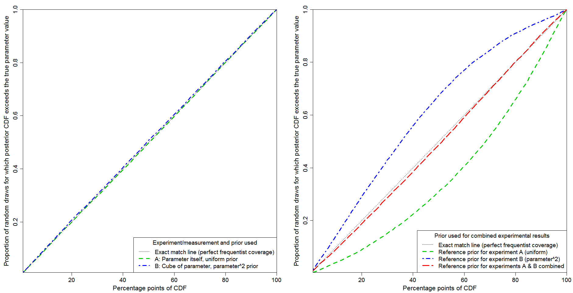
Fig 1: Probability matching for experiments measuring: A – parameter; B – cube of parameter.
The left hand panel relates to inference based on data from each separate experiment, using the correct Jeffreys’ prior (which is also the reference prior) for that experiment. Probability matching is essentially perfect in both cases. That is what one would expect, since in both cases a (transformational) location parameter model applies: the probability of the observed datum depends on the parameter only through the difference between strictly monotonic functions of the observed value and of the parameter. That difference constitutes a so-called pivot variable. In such a location parameter case, Bayesian inference is able to provide exact probability matching, provided the appropriate noninformative prior is used.
The right hand panel relates to inference based on the combined experiments, using the Jeffreys’/reference prior for experiment A (green line), that for experiment B (blue line) or that for the combined experiments (red line), computed by adding in quadrature the priors for experiments A and B, as described above.
Standard Bayesian updating corresponds to either the green or the blue lines depending on whether experiment A or experiment B is analysed first, with the resulting initial posterior PDF being multiplied by the likelihood function from the other experiment to produce the final posterior PDF. It is clear that standard Bayesian updating produces order-dependent inference, with poor probability matching whichever experiment is analysed first.
By contrast, my proposed modification of standard Bayesian updating, using the Jeffreys’/reference prior pertaining to the combined experiments, produces very good probability matching. It is not perfect in this case. Imperfection is to be expected; when there are two experiments there is no longer a location parameter situation, so Bayesian inference cannot achieve exact probability matching.[7]
Numerical testing: Example 2
The second example involves Bernoulli trials. The experiment involves repeatedly making independent random draws with two possible outcomes, “success” and “failure”, the probability of success being the same for every draw. Experiment A involves a fixed number of draws n, with the number of “failures” z being counted, giving a binomial distribution. In Experiment B draws are continued until a fixed number r of failures occur, with the number of observations y being counted, giving a negative binomial distribution.
In this example, the parameter (here the probability of failure, θ) is continuous but the data are discrete. The Jeffreys’ priors for these two experiments differ, by a factor of sqrt(θ). This means that Objective Bayesian inference from them will differ even in the case where z = r and y = n, for which the likelihood functions for experiment A and B are identical. This is unacceptable under orthodox, Subjective, Bayesian theory. That is because it violates the so-called likelihood principle:[8] inference would in this case depend on the stopping rule as well as on the likelihood function for the observed data, which is impermissible.
Figure 2 shows probability matching tested by random draws of experimental results, as in Figure 1. Black dotted lines show perfect probability matching (frequentist coverage).In order to emphasize the difference between the two Jeffreys’ priors, I’ve set n at 40, r at 2, and selected at random 100 probabilities of failure, uniformly in the range 1–11%, repeating the experiments 2000 times at each value.[9]
The left hand panel of Fig. 2 shows inference based on data from each separate experiment. Green dashed and red dashed-dotted lines are based on using the Jeffreys’ prior appropriate to the experiment involved, being respectively binomial and negative binomial cases. Blue and magenta short-dashed lines are for the same experiments but with the priors swapped. When the correct Jeffreys’ prior is used, probability matching is very good: minor fluctuations in the binomial case arise from the discrete nature of the data. When the priors are swapped, matching is poor.
The right hand panel of Fig. 2 shows inference derived from the experiments in combination. The product of their likelihood functions is multiplied by each of three candidate priors. It is multiplied alternatively by the Jeffreys’ prior for experiment A, corresponding to standard Bayesian updating of the experiment A results (green dashed line); by the Jeffreys’ prior for experiment B, corresponding to standard Bayesian updating of the experiment A results (dash-dotted blue line); or by the Jeffreys’ prior for the combined experiments, corresponding to my modified form of updating (red short-dashed line). As in Example 1, use of the combined experiments Jeffreys’ prior provides very good, but not perfect, probability matching, whilst standard Bayesian updating, of the posterior PDF from either experiment generated using the prior that is noninformative for it, produces considerably less accurate probability matching.
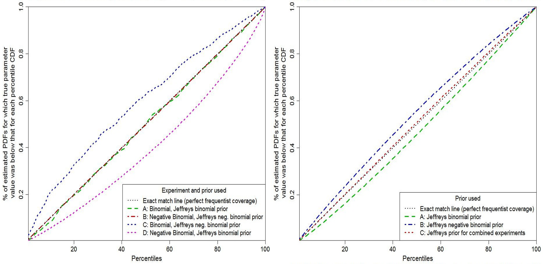
Fig 2: Probability matching for Bernoulli experiments: A – binomial; B – negative binomial.
Conclusions
I have shown that, in general, standard Bayesian updating is not a valid procedure in an objective Bayesian framework, where inference concerns a fixed but unknown parameter and probability matching is considered important (which it normally is). The problem is not with Bayes’ theorem itself, but with its applicability in this situation. The solution that I propose is simple, provided that the necessary likelihood and Jeffreys’ prior/ Fisher information are available in respect of the existing parameter estimate as well as for the new experiment, and that the independence requirement is satisfied. Lack of (conditional) independence between the different data can of course be a problem; prewhitening may offer a solution in some cases (see, e.g., Lewis, 2013b).[10]
I have presented my argument about the unsuitability of standard Bayesian updating for objective inference about continuously valued fixed parameters in the context of all the information coming from observational data, with knowledge of the data uncertainty characteristics. But the same point applies to using Bayes’ theorem with any informative prior, whatever the nature of the information that it represents.
One obvious climate science application of the techniques for combining probabilistic estimates of a parameter set out in this article is the estimation of equilibrium climate sensitivity (ECS). Instrumental data from the industrial period and paleoclimate proxy data should be fairly independent, although there may be some commonality in estimating, for example, radiative forcings. Paleoclimate data, although generally more uncertain, is relatively more informative than industrial period data about high ECS values. The different PDF shapes of the two types of estimate implies that different noninformative priors apply, so using my proposed approach to combining evidence, rather than using standard Bayesian updating, is appropriate if objective Bayesian inference is intended. I have done quite a bit of work on this issue and I am hoping to get a paper published that deals with combining instrumental and paleoclimate ECS estimates.
.
Notes and references
[1] See, e.g., Chapter 5.4 of J M Bernardo and A F M Smith, 1994, Bayesian Theory. Wiley. An updated version of Ch. 5.4 is contained in section 3 of Bayesian Reference Analysis, available at http://www.uv.es/~bernardo/Monograph.pdf
[2] Kolmogorov, A N, 1933, Foundations of the Theory of Probability. Second English edition, Chelsea Publishing Company, 1956, 84 pp.
[3] Kass, R. E. and L. Wasserman, 1996: The Selection of Prior Distributions by Formal Rules. J. Amer. Stat. Ass., 91, 435, 1343-1370. Note that no such conflict normally arise where the parameter takes on only discrete values, since then a uniform prior (equal weighting all parameter values) is noninformative in all cases.
[4] Lewis, N, 2013a: Modification of Bayesian Updating where Continuous Parameters have Differing Relationships with New and Existing Data. arXiv:1308.2791 [stat.ME] http://arxiv.org/ftp/arxiv/papers/1308/1308.2791.pdf.
[5] Barnard, GA, 1994: Pivotal inference illustrated on the Darwin Maize Data. In Aspects of Uncertainty, Freeman, PR and AFM Smith (eds), Wiley, 392pp
[6] In the multiple parameter case, it is necessary to report the Fisher information (a matrix in this case) for the parameter vector, since it is that which gets additively updated, as well as the joint likelihood function for all parameters. Where all parameters involved are of interest, Jeffreys’ prior – here the square root of the determinant of the Fisher information matrix – is normally still the appropriate noninformative prior (it is the reference prior). Where interest lies in only one or a subset of the parameters, the reference prior may differ from Jeffreys’ prior, in which case the reference prior is to be preferred. But even where the best noninformative prior is not Jeffreys’ prior, the starting point for computing it is usually the Fisher information matrix.
[7] This is related to a fundamental difference between frequentist and Bayesian methodology: frequentist methodology involves integrating over the sample space; Bayesian methodology involves integrating over the parameter space.
[8] Berger, J. O. and R. L. Wolpert, 1984: The Likelihood Principle (2nd Ed.). Lecture Notes Monograph, Vol 6, Institute of Mathematical Statistics, 206pp
[9] Using many different probabilities of failure helps iron out steps resulting from the discrete nature of the data.
[10] Lewis, N, 2013b: An objective Bayesian, improved approach for applying optimal fingerprint techniques to estimate climate sensitivity. Jnl Climate, 26, 7414–7429.


36 Comments
I dont want to sound disrespectful but this all sounds like gobbledeegook to me , not being simmered in Bayesian Greek.
A suggestion I would make is , instead of bountiful graphs with “results”, would it be possible to support your text, which no doubt carries a subtle and interesting message but remains entirely unknown to me, would it be possible to support the text with some pictures? Not graphs.Not graphs. Or very few, AFTER we have understood the message.
I feel statisticians dont like picturing what they write. Mathematicians do, engineers do.
I am not sure what where you are and what you want to do.
There must be an “experiment” taken somewhere, I believe, a “model” envisioned” I guess , which is “processed”, but then a “parameter” is changed which lead to maybe other results I do not know.
It would be useful to see some pictures..Just a suggestion.
OT,but Venus, why do you have 6 different websites linked to your name in the last 8 comments you have made?
Tell-tale sign of an absurdist?
Have you bounced this off Andrew Gelman?
No, but he is most welcome to comment on what I have written.
Wouldn’t hurt to contact him directly. I suspect he’d have some comments.
I have now done so.
Statisticians explaining something always gives me this feeling of an art critic pointing to a patch in a Jackson Pollock painting and talking lots and lots about that..it always lacks story and momentum..where is the start what do we want? where do you go with this?
And I think NicLewis is probably the most down to earther amongst them, we should keep him close at heart.
Maybe its the science that does it to them, I dont know? Maybe our machines (who ALL have this theory at their core) will talk like that to us as well in the future??
One of the problems I have with reading statistics is always what movie are they playing in: there are several movies possible.Statistics is the engineering science to try to understand a population, by interpreting a sample. They want to know the populations PDF, most of the time. But most people dont want the pdf at all and are mostly interested in one moment of the MGF that defines the PDF, the average, the result of a measurement.You look at the speedometer of your LADA and want to know if your below 50mph in a 40mph zone..thats the average..a statistician sitting next to you will want to know all the moments, for some reason, but you focus on just one.
They describe methods to each other how to come to a good idea for the population PDF from a sample..thats movie 1.
But they can never “prove” these methods are okay, for that, you need to have a KNOWN population and test the methods on, and see that the method indeed works. thats movie 2.
If you read a bit of staitisticians texts, you never know whether they are in movie 1 or 2.
Nic, could your proposed method be extended to more than just two experiments? To my untrained eye at least, the formula for the combined priors of A and B looks as if one could squarely add a third term under the root. Having available many but small experimental data sets addressing in parts the very same question is just a common case.
Hugo M,
Yes, my proposed method extends to any number of experiments. I referred to combining two or more experiments (with independent data), but I did not amplify how to do so.
Provided Jeffreys’ prior is the appropriate noninformative prior, one can do this sequentially, provided that after each experiment is analysed the combined likelihood function and the Jeffreys’ prior is made available, not just the posterior PDF. Updating with the results of the new experiment then simply involves multiplying the existing combination likelihood function by the new experiment’s likelihood function, and adding in quadrature the Jeffrey’s prior for the new experiment.
If the parameter is multivariate, the full Fisher information (here a matrix) for the existing combination of experiments needs to be made available, and the Fisher information for the new experiment added to it. Jeffreys’ prior can then be derived as the square root of the determinant of the updated Fisher information matrix.
Alternatively, and equivalently, one could analyse all the experiments simultaneously, computing the likelihood and Fisher information for each, and then combine their likelihood functions multiplicatively and their Fisher informations additively. The combined experiments posterior PDF is then the product of the combined likelihood function and the applicable Jeffreys’ prior – which is the square root of the combined Fisher information (of its determinant in a multiparameter case).
If Jeffreys’ prior is not the appropriate noninformative prior, the combined Fisher information should still be calculated, and the desired prior calculated using it and any other required details of the experiments.
Nic,
Thanks for the detailed posting! (You’ve raised the level of discussion a couple of notches with this series: far above any other climate blog on either side of the debate.)
I’ve read your Example 1 a couple of times and your paper and still can’t figure out what’s happening in the non-Jeffry’s-prior case:
A) Are you using uniform priors for experiment A (when first) or experiment B (when first)? If so, this seems to be more of a uniform v. most-anything-else discussion instead of a subjective v. objective discussion.
B) How are you combining $param$ and $param^3$? You’re not combining the probability densities directly — which wouldn’t make sense considering one is the cube of the other — but I can’t quite figure it out. Are you interpolating your two densities to account for the x-axis being the cube or cube root, or something else?
Thanks! To answer your questions re Example 1:
A) I use a uniform prior for experiment A when it is analysed separately, as a uniform prior is completely noninformative (and is the Jeffreys’ prior) when estimating a parameter measured with Gaussian or similar errors. I also use therefore a uniform prior when combining information from experiments A and B by standard Bayesian updating, with A analysed first, since in that case the posterior PDF for experiment A using a noninformative uniform prior for it is updated by using it as the prior and multiplying it by the likelihood function for experiment B, in a further application of Bayes’ theorem. Doing so gives the green dashed line in the RH panel of Fig. 1.
I use a parameter^2 prior for experiment B when it is analysed separately, as that prior is completely noninformative (and is the Jeffreys’ prior) for estimating a parameter when the cube of the parameter is measured with Gaussian or similar errors. I also use therefore a parameter^2 prior when combining information from experiments B and A by standard Bayesian updating, with B analysed first, since in that case the posterior PDF for experiment B using a noninformative parameter^2 prior for it is updated by using it as the prior and multiplying it by the likelihood function for experiment A, in a further application of Bayes’ theorem. Doing so gives the blue dashed line in the RH panel of Fig. 1.
What these two ways of combining information illustrate is a naïve objective Bayesian approach: the initial prior used is noninformative, but it is in effect also used as the prior for the combined experiment likelihood function, for which it is not noninformative. I don’t regard this as a subjective Bayesian approach: although a subjective Bayesian might well choose a uniform prior for analysing experiment A, but probably not because it was the Jeffreys’ prior.
B) What is measured in experiment B is the parameter cubed, but the estimate for the parameter is the cube-root of the measurement. For example, the parameter might be the diameter of a sphere, the volume of which is measured with a Gaussian distributed error in experiment B. In experiment A, the diameter itself is measured. I don’t need to interpolate. In experiment B, the likelihood as a function of the parameter itself is readily obtained by using −0.5*([Measured volume − (pi/6)*parameter ^3]/Error standard deviation)^2 as the exponent in the Gaussian density function. Although expressed as functions of the parameter, with the data fixed at its realised (measured) value, likelihood functions are probability densities for the measured data variable, not for the parameter.
it very well might be that a Jeffreys Prior allows for “invariance” when considering p p^2 in a bernouilli.
But it will come at a COST.
It is HARMFUL NONSENSE to modify experimental results for the sake that you will want to “modify” what you wished to measure in the first place. The discussion of sdvariance with normal distributions is the classic NONSENSE in this.
What I lack in the discussion is the COST of the introduced sophistry.
Also it looks to me that you are NEVER going to achieve a “prior” for all possible imaginable parameter transformations. This is where you are going to say you just “maximise” a little Fisher info or whatever..but what
does THAT mean, really? cocktail mixing the data a little.
Note the JP in the Keenan discussion isnt anything “prior” at all is it.
Thats a plain probability map, and Jeffrey should NEVER have called that an “objective prior”..probability theory preceded him, and its a formal maths theory unlike his voodoo.
I should add i dont understand most/any of this prior theory at all.
a “measurement” in my eyes is a PDF. PDF and MGF are one to one.
In principle PDF contains all moments. p, p^2, p^3 up to infinity, and you can mix and match them.
so what IS the meaning of modifying the measurement to allow for “invariance” of some of the moments?
venus
I am afraid your comments make little sense and are not helpful to a serious discussion of these issues. In the interests of other readers and those who wish to contribute to a sensible discussion, I shall be obliged to snip any further such comments from you.
Venus, Nic is a very politely man, an English gentleman. I’m not from there… so I would like to express it in this way: You write: ” I should add i dont understand most/any of this prior theory at all.” This is not a shame, but why do you make a post describing your incompetence on this field? Must everybody post about things he doesn’t understand? Silence is golden!
Hi, as requested I am giving a comment.
Nic Lewis wrote, “I compared Subjective Bayesian methodology based on a known probability distribution, from which one or more values were drawn at random, with an Objective Bayesian approach using a noninformative prior that produced results depending only on the data and the assumed statistical model.”
But I don’t really buy this “subjective” vs “objective” thing. _Any_ Bayesian method will give results depending only on the data and the assumed statistical model. There is no general subjective choice of model, nor is there any general objective choice of model. Either way you just have to put down a model and go from there, work out its implications and check the model where possible. The model to which I refer includes data model and prior distribution.
For readers interested in more on this topic, I recommend chapter 1 of our book, Bayesian Data Analysis.
Nic also asks: “a) what prior you would use when estimating a parameter the value of which is observed with an error distribution known to be Gaussian with zero mean and known standard deviation, where there is no other known information that bears on the parameter value; and b) how you would update your posterior PDF if the value of the parameter cubed was then observed with an error distribution known to be Gaussian with zero mean and known standard deviation?”
My response is: (a) the prior distribution I would use will depend on the problem, just as my data model will depend on the problem I am studying, (b) I would update the posterior distribution using the usual Bayesian rules, and (c) I don’t think it’s typically realistic that your error distribution is known.
Andrew Gelman,
Thank you for your contribution, but it does seem to me to be at best a political response and at worst a non-response. Do you have a preferred answer to the specific problem posed?
Kribaez:
I think you misunderstand. Nic Lewis emailed me asking for my reactions to his post and he followed up with a couple of questions. At his request, I posted my response in the comments section here. There is no political content to my response–it is entirely statistics.
+1
Andrew,
Many thanks for commenting. I agree that it is not always clear what choice of prior distribution is most objective, in the sense of being least informative (least affecting inference), when using an objective Bayesian approach. But I do think that there is a difference between subjective and objective Bayesian approaches to parameter estimation, as regards the prior distribution component of the statistical model.
Subjective Bayesians regard the prior distribution as having a direct probabilistic interpretation, as representing existing beliefs about a parameter. By contrast, most objective Bayesians regard the prior as simply a weight function, not having any direct probabilistic interpretation, that results in generation of a posterior PDF that has desirable characteristics. So, Bernardo & Smith (Bayesian Theory,1994) say that their reference prior is “simply a mathematical tool” and make clear that it has no direct probabilistic interpretation.
Likewise, Fraser and Reid (e.g., On default priors and approximate location models, 2011) refer to using mathematical priors to weight likelihood functions. They also state clearly what Bernardo and Smith admit only implicitly, that the probability lemma for calculating conditional probability from two probability inputs does not apply when there is only one probability input available, and hence Bayes’ theorem does not apply when no genuine probabilistic prior is available.
For readers interested in learning more about objective Bayesian inference and noninformative priors, Kass & Wasserman (1996: reference [3] above) gives a good introduction to the subject. I have found the reference analysis chapter of Bernardo & Smith (1994: link given in reference [1] above) gives a very useful, if somewhat technical, explanation of objective Bayesian inference, albeit focussed on the development of reference priors. And Don Fraser’s various papers (e.g., “Is Bayes Posterior just Quick and Dirty Confidence?”, Statistical Science, 2011) contain deep insights into the issues involved.
Regarding your answers to my specific questions:
(a) Could you clarify what aspect of the problem I had not specified well enough for you to be able to say what prior you would use, and give me an example of a case within my specifications where you would not use a uniform prior covering the whole real line?
(b) Your use of the standard method of Bayesian updating, adopting the existing posterior as the prior, for inference about a fixed but unknown parameter is a clear distinction between our approaches. Obviously, yours is very much the generally accepted view at present.
(c) You may well be right in general about error distributions not being known. Estimation of climate system parameters is probably unusual in that the observational record is generally insufficiently long to permit estimation of internal climate variability from observations, and observational uncertainty is typically difficult to estimate directly from observational data. Instead, separate plug-in estimates of internal variability and observational uncertainty taken from other sources are typically used, with either Gaussian or t-distributions usually being assumed.
If the question here is whether a Bayesian prior can be selected that supports a political posterior, that has been answered in the affirmative by Nic’s analyses and publications on the use of a uniform prior in Bayesian analysis of ECS. You do not need Andrew Gelman to settle that issue. Can a scientific community maintain that prior and political posterior without objection – other than Nic’s. Unfortunately that apparent abuse of Bayesian analysis can be maintained.
On the other hand, the issue of objective and subjective priors as argued by Nic here has implications that go to the heart of the basis of Bayesian analysis or at least that part that is termed subjective. That issue could well call for an expert opinion.
Nic —
The examples you give here present interesting problems for prior selection, but don’t relate to the Radiocarbon calibration problem you raised anew in your March 2 post. In my last comments there, I argued that you get the same results whether you lump data sets A and B (calibration data and sample data) or first incorporate A and then use its posterior as the prior for B.
Your Example 1 presents an interesting, if artificial, problem for the Jeffreys information prior, since data sets A and B use the parameters in a different way. As a result, the Jeffreys prior for A and B together appears to be different from that for data set A by itself. I’m not sure how one should deal with that. However, the nonlinearity in your example is an assumed part of the model, not an outcome of the data as in the Radiocarbon calibration case.
I’m not convinced that your Example 2 would require different priors for the two experiments, however. In the first experiment, z has a binomial distribution given the number n of draws and the probability theta of failure. The Jeffreys Information prior (If I’ve done this right) is then proportional to (theta (1-theta))^(-1/2) (and not 1/((theta (1-theta) as Jeffreys actually advocated, according to Zellner’s Intro to Bayesian Inference, p. 40). But I don’t see why you’d get any different prior for the second experiment, since the underlying Bernoulli process is exactly the same. If for some reason the probability of a single failure in the second experiment was the square of that in the first experiment, there would be an issue like in your Example 1, but that is not the case.
Applying Jeffreys to the Radiocarbon calibration problem is unusual, in that before any data is observed, the expected log likelihood is constant for all t (all t less than the present, anyway), and therefore the information is zero throughout. This isn’t necessarily the same thing as being a constant throughout, but still it doesn’t argue for a non-constant.
Hu,
You’re right, this article is not directly related to the radiocarbon calibration problem.
In Example 1, the Jeffreys’ prior for analysing experiments A and B together really is different from the Jeffreys’ prior for experiment A on its own (or experiment B on its own).
Re Example 2, it is well established that the Jeffreys’ prior for an experiment with a fixed number of Bernoulli trials, which gives rise to a binomial distribution, differs from that for an experiment where the required number of failures (or successes) is specified, which gives rise to a negative Binomial (Pascal) distributions. I first came across this in Box & Tiao’s excellent 1973 book ‘Bayesian inference in statistical analysis’ (p.45). In the first case, the Jeffreys’ prior is: (theta (1 − theta))^ −0.5, where theta is the probability of failure, as you say. But in the second case, Jeffreys’ prior is: theta^ −1 (1 − theta)^ −0.5.
The reason for the difference is that although, if the number of trials and of failures is the same in each case the two likelihood functions are the same, determining the expected Fisher information involves summing over different sample spaces (the number of failures in the binomial case, but the number of trials in the negative binomial case). As a result, the Fisher information differs, and hence so do the Jeffreys’ priors.
Nic —
Thanks for the information. I suppose that the negative binomial might provide different information, since we know for certain that the y-th draw was a failure. Yet all draws were independent with the same probability of failure ex ante in both experiments, so this is still counter-intuitive to me.
If we use the Jeffreys Info prior beta(.5, .5) for the binomial experiment, and have z failures in n draws, the posterior is beta(.5+z, .5+n-z). What is the posterior for the negative binomial experiment if we start with beta(0, .5) and observe that it takes y draws to get r failures? Does it turn out to be the same despite the different prior?
Although Arnold Zellner (every Chicagoan’s Bayesian guru, sadly deceased in 2010) presents the Jeffreys Info prior in his 1960 text, he relegates it to an appendix. He points out that although it gives a reasonable uniform prior for a pure location parameter problem, and a reasonable 1/s prior (which is uniform in log s) for a pure scale (s) parameter problem, in the important case in which both location and scale are unknown, it unreasonably gives a 1/s^2 prior (since |I| then picks up 1/s^2 from both the location and scale elements of the Information matrix). I am therefore now likewise wary of a strict Jeffreys Info prior.
For the binomial problem, Zellner endorses the beta(0,0) prior preferred by Lindley and by Jeffreys himself despite its non-conformity with Information criterion, on the grounds that it gives a uniform distribution for the log odds ratio log(theta/(1-theta). He does not even mention the beta(.5, .5) prior that does follow from the JI criterion, but I’m actually beginning to like that one, since it does have a theoretical basis, and gives a less dogmatic posterior when the data is all one way or the other: With n draws and 0 failures, a beta(0, 0) prior leads to a beta(0, n) posterior, which is massed at theta = 0 with no room for doubt. But beta(.5, .5) leads to beta(.5, n+.5), which has mean .5/(n+1). This is virtually 0 if n is large, but does not purport to be certain. The Bayes-Laplace beta(1,1) = U(0,1) prior is likewise non-dogmatic in this case, but is a little arbitrary.
Hu,
Regarding the posteriors, if y = n and z = r then the likelihood functions in the two cases are identical, so the negative binomial experiment posterior differs from the binomial experiment posterior by the same multiplicative factor as the difference in their Jeffreys’ priors, being theta^ −0.5. In your example, the posterior for the negative binomial experiment using its beta (0, .5) Jeffreys’ prior would be beta(r, 0.5 + y − r).
I’m a fan of Zellner too – his 1971 book “An introduction to Bayesian Inference in Econometrics” is an excellent primer on objective Bayesianism. Jeffreys’ himself realised that the strict Jeffreys’ prior was not always appropriate when multiple parameters were being estimated but inference was required about one of them (or a subset of them) in isolation. His solution was the Jeffreys’ independence prior, constructed by treating independent parameters separately and multiplying the Jeffreys’ priors pertaining to each of them individually. So, in the location–scale problem you mention, the resulting prior would be the product of the uniform prior for the location parameter and the 1/s prior for the scale parameter, being 1/s. The problem with the strict Jeffreys’ prior arises here because the standard deviation (s, the scale parameter) affects the precision of the estimate of the mean (μ, the location parameter) and hence appears in its prior (which is uniform in μ, but with a value of 1/s). When the joint Jeffreys’ prior for (μ, s) is computed that factor of 1/s, which is only relevant to estimating μ, gets combined with the 1/s factor that is required for correctly estimating s.
The problem is arguably more to do with the marginalisation process used to form a posterior for each parameter on its own, by integrating out the other parameter, than with the Jeffreys’ prior itself. The best solution in such cases is normally to use a right Haar prior, where a suitable transformation group relationship exists between the parameters, or to use Jose Bernardo’s more complex reference prior approach. Such reference priors are often regarded as the ‘gold standard’ by objective Bayesians. They equate to Jeffreys’ prior except where inference is required about a subset of multiple parameters. In such cases, they normally equate to the right Haar prior where that exists, but otherwise they may depend on which parameter(s) of those being estimated are of particular interest.
In the areas of climate science that I have been involved in, the basic Jeffreys’ prior usually seems suitable, probably because plug-in uncertainty estimates are used rather than standard deviations being estimated simultaneously with the central value.
IMO the strict Jeffreys’ prior is preferable for the binomial problem. As I show, it gives rise to essentially exact probability matching, which other priors therefore will not. It is also the reference prior, of course. Bernardo and Smith’s Bayesian Theory book recommends Geisser (1984): On prior distributions for binary trials, J Amer Stat Assoc, with discussion, for further reading about this problem.
Thanks, Nic. It looks like I’ll have to read up on Bernardo reference priors now!
BTW, the correct date for the Zellner text I was citing is indeed 1971.
Reblogged this on I Didn't Ask To Be a Blog.
There are several ways to proceed with Bayesian analysis , depending on the situation. Suppose the data model is not in dispute and you have a large amount of data. Then it will often be the case that the data overwhelm the prior and the posterior is insensitive to the prior. In this case, the prior is moot. If there is less data and different reasonable priors result in significantly different posteriors, then the lack of data (information) to overwhelm the prior is an inherent property of the study and no efforts should be made to obscure that fact. In this case, reasonable people can engage in scientific discourse to discuss their beliefs and understandings of the prior. Also, more data can be collected. If the data model is in dispute to the degree that different models result in significantly different posteriors, then a similar situation obtains and the data model should be disputed. That is, Bayesian analysis has identified the locus of scientific uncertainty and disagreement. In my perusal of climate studies as discussed on this website, I have often felt that climate scientists have assumed simplistic data models and not given sufficient attention to their validity.
rwnj, thanks for your comment.
Unfortunately, in many cases in climate science the data is poor and it is not practicable to improve it by obtaining more data – unless someone invents a time machine!
You say “reasonable people can engage in scientific discourse to discuss their beliefs and understandings of the prior.” However, I believe that the only valid purpose of the prior is to convert the likelihood function into a posterior PDF. If there is genuine existing knowledge, it needs to be represented as a likelihood function (to be combined with the likelihood function for the experiment being analysed, with which it may also be compared) not as a prior PDF. This view is, of course, anathma to most Bayesians, but I am confident that it will in time be seen to be correct.
I don’t disagree that cliamte scientists may often have over simplistic data models. But in the area of climate sensitivity estimation that i am most involved with, differences in estimates have mainly arisen either a) because different data sources, with notably different values, have been used (e.g., for aerosol forcing); or b) because different statistical methods have been used – mainly subjective Bayesian methods with a uniform or “expert” prior on the one hand, or either frequentist (including likelihood ratio) methods or (in the case of my studies in particular) objective Bayesian mothods with a noninformative prior on the other hand.
Nic Lewis, I have reposted this from the next thread on Gavin Schmidt:
May I recommend the book “A Comparison of Frequentist and Bayesian Methods of Estimation” by Prof Francisco Samaniego?
Short take-home message: the asserted superiority of Bayesian methods depends on the accuracy of the prior. He calls it a “threshold” that must be met for the Bayesian method to be better than the frequentist. He provides a Bayesian metric for assessing goodness.
Also, it may or may not be true that that a 0 value for a parameter is highly unlikely; but it is demonstrably true in many settings that parameter values really, really close to 0 are sufficiently accurate. Take, for example, the effects of most gene expression levels on most measures of health and disease: it might be called a vast desert of true nil null hypotheses.
I read CA now and then. You write at a uniformly high standard. Please keep up the good work.
Your title says: “Incorporating prior information “. Do you think that “prior information” ought to have been subjected to stringent testing like most other claims about the world? Has anyone shown that the mean of the posterior distribution calculated from using a Jeffreys prior converges to the true value faster than the maximum likelihood estimator from the same likelihood function as used there? Unless the prior has a mean equal to the true value, the mle will converge to the true value faster than the mean of the corresponding posterior distribution.
matthewmarler, thank you for your comment.
Just to clarify, I have focussed on estimation of parameter values rather than hypothesis testing.
The prior information that I am thinking of is information derived from observations, so is of the same nature as information derived from the new dataset being analysed. So logically their reliability should be tested in similar ways.
Bayesian parameter estimation isn’t focussed on obtaining a point estimate, but when one is wanted it is generally better to use the posterior median, which is invariant under reparameterisation, than the posterior mean (or the posterior mode), which is not.
“Unless the prior has a mean equal to the true value, the mle will converge to the true value faster than the mean of the corresponding posterior distribution.”
If a noninformative reference prior is used (being Jeffreys prior, in the univariate case) – which will often have no finite mean – then I believe the mle and the posterior distribtion will converge at the same rate to the true value of the parameter. See Bernardo and Smith, 1994, Appendix B.4.4.
Just to clarify, Samaniego’s book is about parameter estimation. And the mle converging faster to the true value is a statement about the relative accuracies of the corresponding confidence intervals and credible intervals. Unless the “threshold” criterion is met, for large N the confidence intervals will be more credible than the credible intervals.
About this: Bayesian parameter estimation isn’t focussed on obtaining a point estimate
Everyone in science wants accurate point estimates. Invariance under transformations is generally disparaged by Bayesians when it is applied by frequentists. It’s the posterior mean about which you can prove it has a smaller mse than the mle, in appropriate cases.
Why use noninformative priors if the goal, as stated in your title, is to incorporate prior information.
These Critical comments aside, I respect your work.
“Why use noninformative priors if the goal, as stated in your title, is to incorporate prior information.”
Because in my view prior information about a fixed but unknown parameter needs to be conveyed by a likelihood function, not by a prior distribution. I believe that standard Bayesian theory in this respect does not in general lead to objective inference (at least in long run probability matching terms). The true function of the prior, if you are looking for objective inference, is to convert a density in data space – the likelihood function (whether from one experiment or two or more experiments combined – into a density in parameter space. That is, in essence, what a noninformative prior does.
About this: I believe the mle and the posterior distribtion will converge at the same rate to the true value of the parameter. See Bernardo and Smith, 1994, Appendix B.4.4.
This they converge at the same rate, but above a certain sample size, the mle is always almost surely closer to the true value than the posterior mean.
oops, “Yes” they converge at the same “rate”.