A guest article by Frank Bosse (posted by Nic Lewis)
A recent paper by the authors Stolpe, Medhaug and Knutti (thereafter S. 17) deals with a longstanding question: By how much are the Global Mean Surface Temperatures (GMST) influenced by the internal variability of the Atlantic (AMV/AMO) and the Pacific (PMV/PDO/IPO)?
The authors analyze the impacts of the natural up’s and down’s of both basins on the temperature record HadCRUT4.5.
A few months ago this post of mine was published which considered the influence of the Atlantic variability.
I want to compare some of the results.
In the beginning I want to offer some continuing implications of S. 17.
The key figure of S. 17 (fig. 7a) describes most of the results. It shows a variability- adjusted HadCRUT4.5 record:
Fig.1: The Fig. 7a from S. 17 shows the GMST record (orange) between
1900 and 2005, adjusted for the Atlantic & Pacific variability.
Unfortunately I couldn’t find the data, therefore I digitized the orange graph and synthesized the annual data. Foremost I wanted to check this sentence from the conclusion:
“With a contribution of less than 10%, the measured global warming during the second half of the 20th century is not much affected by Atlantic and Pacific variability, underlining that most of this observed warming is caused by anthropogenic forcings.”
At first I calculated the regression of the variability adjusted HadCRUT4.5 record on the forcing (IPCC AR5), which is very impressive:
Fig. 2: The correlation between the forcing and the Temperature change
of S 17. 91% of the temperature variance is due to the forcing changes.
The unadjusted HadCRUT4.5 record (also from 1900…2005 and smoothed with a 10-year loess) gives R²=0.85. This implies for the whole time span: 6% of the variance of the temperatures is due to the AMV&PMV, calculated in S.17.
The slope of the linear Trend (multiplied with 3.71 W/m² for the IPCC forcing due to 2*CO2) results in a TCR of 1.35 K, for the unadjusted record of HadCRUT4.5 it’s almost the same value: 1.36 K. This is no surprise because over the long time span the influence of the decadal variability will cancel out.
The cited sentence from the conclusions in S.17 is valid only for the second half of the 20th century.
Therefore I calculated the slopes (see Fig.2) for every year from 1950 to 1976 with the constant end year 2005 and multiplied them with 3.71 to estimate the TCR.
Fig. 3: The TCR to 2005 calculated for each year from 1950 to 1976 with the results of S.17
Note in Fig.3 that the TCR of the adjusted record is relatively flat till around 1970 in contrast to the unadjusted record. For the S.17- adjusted record of HADCRUT4.5 the TCR from 1970 to 2005 is 1.33 K. For the unadjusted HADCRUT4.5 this value is 1.74 K. The reduction is due to the internal variability of the oceans as it was calculated in S 17. The relative difference of the TCR values:
Fig. 4: The percentage of the influence of AMV and PMV on the TCR after 1950 following S.17.
If one interprets the cited sentence from the conclusions of S.17 literally, it’s correct: the second half of the 20th century began in 1950 and the influence on TCR in S.17 is well below 10% (it’s 7%). For the more critical years for the tuning of the CMIP5- models after 1970 it reaches up to 24%. This overestimation is the result of the AMV&PMV as the result of S.17 shows. The mean TCR in the CMIP5 models is 1.8 K.
Comparisons with the formerly proposed method
In the time since the release I considered some new findings from the literature and advanced some details.
- Selection of data
GMST: In S.17 they use HadCRUT4.5 as the temperature record. This is questionable due to some gaps in the spatial coverage of this record. In this blogpost Nic Lewis examined the GISS-record and recommended the record of Cowtan/Way for model vs. observation comparisons. In the following discussion it was mentioned that the BEST record is also very helpful. Therefore I use the average of both records.
Atlantic variability: In S. 17 they use an Index from this study. There are some disadvantages from the inclusion of the tropical part of the Atlantic it’s shown in v. Oldenborgh et.al (2009). Therefore I use the SST 25…60°N; 70…7°W (HadSST3) regressed on the forcing (NOT on the GMST) to generate the AMO index.
Forcing: The basis is the record of the IPCC (AR5). In the following years some improvements were released ( see here and here ) which are now included in the used forcing-record. The volcano forcing is excluded for all calculations.
- The internal variability of the GMST
The GMST are regressed on the forcing for the time span from 1871 to 2016 with annual data. The residuals of this regression:
Fig. 5: The unforced variability of the GMST (GMSTV) filtered with a 10a-Loess smoother. One can
notice that the volcanic influence and the ENSO-imprints are relatively small due to the smoothing.
The regression of the GMSTV on the AMO record (see fig. 3 of the discussed post) shows a significant trend:
Fig. 6: The relationship between the GMSTV and the AMO with annual unsmoothed data.
In S.17 they also include the Pacific Internal Variability. The authors use the Tripole(IPO) Index . Unfortunately I could not find any statistically valid inference between this index (and also the PDO index) and the GMSTV which also rises some doubts on the results of this recent paper . Therefore I wasn’t able to include a decadal Pacific variability due to the lack of any significance.
- The TCR-estimation after removing the Atlantic internal variability
After removing the weighted AMO Influence (see Fig.6) on the GMST the adjustment shows this result:
Fig. 7: The raw- and AMO-adjusted GMST filtered with a 10a Loess smoother. Note that the longtime trend is not influenced and that the adjustments produce only a difference of about 0.1K at maximum. The often discussed “hiatus” vanished.
For the estimation of the TCR in the years with stronger forcing from 1950 and following I calculated the trends of GMST vs. Forcing to the constant end year 2015. The year 2016 is excluded as it was strongly influenced by an ENSO-event (see Fig. 5). To calculate the TCR from the feedback I multiplied these lambda-data with 3.8W/m² for a doubling of CO2.
Fig. 8: The TCR estimated from the raw GMST and AMO adjusted GMST. Observe the stability
of the TCR with no significant trend. The mean for the calculated trends from 1950 to 1985
with the end in 2015 gives 1.29 +-0.04 K/2*CO2 with 95% confidence (2*Sigma).
A more detailed uncertainty analyses which would also include the GMST, Forcing- and AMO- uncertainties is beyond the scope of this post .
Finally I calculated the percentage of the influence of the variability on the TCR to compare it with Fig.4.
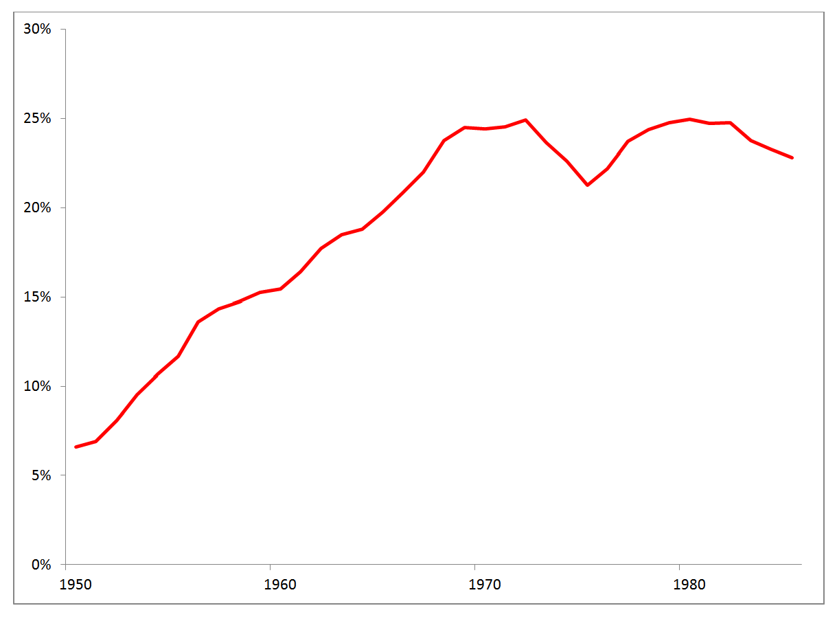
Fig. 9: The percentage of the influence of the variability on the TCR. Note the similarity in the years to 1970
to the estimation included in S.17. The longer record (to 2015) makes the estimation more valid up to 1985.
Conclusion
Considering the internal variability reduces the calculated TCR for the years after 1970 by about 25%. It solves the problem, that the TCR is significant lower for the time span 1950…2015 than for the time span 1975…2015.
The inclusion of the Pacific decadal variability does not improve the result, confirming some recent findings.
This actual paper about the west-tropical Pacific confirms the “Iris-effect” from observations with the implication that the ECS is estimated at about 2K for the doubling of CO2. Into the same direction points this study about the mid-latitude cloud response to the forcing. The discussed result from this post seems to be also a strong argument for a sensitivity of the GMST to Carbon Dioxide at the lower end of the IPCC AR5 1.5-4.5 K range.
Note: Frank Bosse and I have been cooperating in investigating isolating the impact of Atlantic multidecadal variability (AMO/AMV) on TCR estimation. This post reflects an approach that we both consider to be defensible; it removes any anthropogenic forcing signal from the measure of AMO/AMV. English is not Frank’s mother tongue, so please avoid criticisms about English language usage, except where something is unclear. Nic Lewis


59 Comments
Frank, I have read your post with interest since it is somewhat along the lines I have been pursuing in decomposing the global mean surface temperatures (GMST) for both observed and modeled series and thus thought you might be interested in commenting on some work I have been doing with observed and modeled GMST series using a relatively new method known as Ensemble Empirical Mode Decomposition (EEMD). A summary of my work with EEMD is linked in a this post as a Word document.
I am of the view that the recent global warming is caused partly by anthropogenic and partly by natural effects and that the big question going forward is the relative portions from these two sources. Estimations of the sensitivity of temperature to radiative forcings, and particularly anthropogenic sourced green house gases, from observations and for determining the validity of climate model output depend critically on estimating these portions.
If there are methods available for demonstratively improved separation of the global warming series components and to thus better estimate these portions – such as the methods EEMD/ CEEMD – then one has to wonder whether the seeming lack of interest by the climate science community to this newer approach is due to unfamiliarity with that method. I make no claims of originality, novelty or propriety for my work presented here, but rather put it out with hopes of getting the climate science community interested in looking further into this approach and its application to temperature series.
https://www.dropbox.com/s/axg9xxzyzwmyrhd/Summary_EEMD_for_Hausfather_Cowtan.docx?dl=0
Frank/Nic I have a post in moderation with a single link. I think the post is most pertinent to Franks\’s thread here.
Ken Fritsch
Now released
With respect to removing the anthropogenic signal to get your AMO index… One problem is that temperatures are not only influenced by forcing, but also the fact that there is a delayed response to forcing. So maybe for your regression, in addition to having forcing as an independent variable, include some forcing variables that have an exponential time lag. Alternatively, perhaps you could deal with this issue in another way, such as adding a low order polynomial of time (quadratic or cubic should be enough) to the regression.
If you ignore the effect of delayed response to forcing, then I think your results will overestimate the impact of AMO on global temperatures.
Also, it would be nice if either you or Nic Lewis could elaborate on the merits of detrending using forcing instead of GMST.
-1: Yes, the SST response to forcing is indeed delayed, with a time constant of several years. I have tried regressing SST on forcing with an exponential delay of a few years. It makes little difference to the residuals (the AMO signal) when anthropogenic forcing is the regressor, as the forcing signal is smooth and only changes slope very slowly.
The main difference between regressing on forcing and regressing on time (linear detrending, as done in the well known NOAA AMO index) is that the faster growth of forcing in recent decades compared with earlier in the record tends to exaggerate the positive recent AMO signal.
I don’t think anyone detrends using GMST to obtain the AMO.
-1: About the advantage of using the forcing and not GMST for the AMO index: If one wants to conclude the influence of the Atlentic variability on the GMST and uses the GMST also for the construction of the AMO index this would be a circular reasoning wouldn’t it?
Post says: “The volcano forcing is excluded for all calculations.”
Can you elaborate on the effects of volcanic and other aerosols on the calculations?
Is it possible that some of the early 20th century warming was not from anthropogenic forcings? Is so, is there a strategy to isolate it?
Ron, the impact of aerosol forcing is included but not the volcano forcing. It’s very strong in relation to the other forcings in the used forcing record. For the estimation of the TCR after 1950 ( see fig. 8) it would introduce a bias because there were no events with bigger impact on the stratosphere after 1993.
Frank, thanks for your explanation. When you say “It’s very strong in relation to the other forcings” do you suspect that volcanic forcing is overestimated by the CMIP5 models?
Also, following on Ken Fritsch’s question and my own, do you have any intentions of trying to isolate Anthro from natural effects that are non-oscillating? For example, the polar ice extents affect albedo and thus can provide a feedback that runs independently from a variation in ocean overturning or AGW.
Ron: The volcano forrcing is perhaps indeed ( by about 50%) overestimated. The other reason for excluding it was the possible bias as I mentioned obove. For oscillating: It’s unclear up to now if the Atlantic variability is an oscillation in the sense of this wording. AMO is the traditionally term therefore I used it. And no: For the closer future I don’t have any intention to separate Anthro from other natural variabilities because the AMO(AMV) seems to be the most important variability. focus on the core…
I guess that using forcing instead of GMST also avoids any issue of reverse causality.
With respect to avoiding volcano forcing… Doesn’t the fact that the AMO residual appears to have no significant relationship with volcanic forcing indicate that using forcing with no time lag is incorrect?
Perhaps it would be better to use overall forcing (with volcano forcing included) and introduce a single exponential time lag, where the decay rate is optimized via least squares. In this way, volcano forcing can be used to determine the appropriate time lag.
-1: Your idea sounds good but is likely to produce invalid results in practice. Whilst anthropogenic forcings appear (at least on average) to have unit efficacy, volcanic forcing only has an efficacy of ~0.5 w.r.t. its RF. And because it is very variable albeit low in mean amplitude, it tends to dominate the fits when OLS (or any other L2 error measure based method) regression is used.
As I wrote before, ignoring the decay time when estimating the fit has very little impact on the residuals.
-1: I’m not quite sure what you mean with “AMO residuals”, if you mean the unsmoothed GMSTV ( the residuals of the regression of the GMST vs. Forcing) has significant relation to volcano events but the smoothing makes ist small. Anyway, not sure if I understood your question correctly.
@ nic, in that case, what if you had both non-volcanic and volcanic forcing as separate independent variables in your regression, but gave them the same exponential time lag? That way, you can allow for significantly different forcing efficiency, but also take advantage of volcanic forcing to try to determine the optimal time lag.
-1: perhaps you’ld like to try doing so, as it is your suggestion?
That’s why we post code and data.
Some years ago, I used an empirical decomposition of a temperature series to isolate the long-wavelength (or secular) trajectory, and then forward-modeled the system under two assumptions (i) that the multidecadal variations were unforced redistributions of internal heat aka “natural internal variability” and (ii) that they were forced variations caused by an unknown oscillatory forcing.
I used a two-body EBM. For case (ii), I back-calculated the level of oscillatory forcing required to induce the temperature oscillation assuming the same level of efficacy as the “known”, input radiative forcings.
My first conclusion would confirm the finding of this study – TCR estimates are robust to inclusion/exclusion of the multidecadal oscillations.
I found in addition that effective ECS is also relatively insensitive to assumptions about the multidecadal cycles – tested over a range of ocean heat datasets. Specifically, for the same ocean heat dataset, including or excluding the effect of the multidecadal cycles, whether as unforced natural variation or forced cycles, makes little difference to ECS estimation, provided the test is over a long-enough timeframe.
While this is a useful thing to know, I believe that it only scratches the surface of the true underlying problem, which is that the available data strongly suggest the existence of a major paradox in climate science.
Basic predicates of modern climate science are:-
a) Energy superdominantly enters and leaves the system radiatively. (Other known and unknown fluxes are negligible.)
b) We can identify a set of radiative forcing drivers which are exclusive and exhaustive.
A corrollary to the above two predicates is that, since you cannot induce a periodic net flux and temperature response without an input radiative forcing of the same periodicity, that the quasi-60 year variations in net flux, temperature (as well as wind systems, cloud and albedo variation) must be attributable to spontaneous internal unforced natural variation. (As an aside, it is worth noting that no AOGCM has been able to reproduce the periodicity and amplitude of these variations.) This is absolutely contra-indicated by the data we have available, and specifically by the relative phasing of the variation in net flux and temperature.
A simple single-body heating model, forced by an oscillatory input flux forcing will always result in a net flux which leads the temperature response by 90 degrees or pi/2 radians phase shift. A more complex heating model – a mixed layer plus deep ocean two-body model, say – will result in a relative phasing between net flux and temperature which is theoretically limited to a maximum of 90 degrees separation. On the other hand, with unforced redistribution of internal heat, theory says that as surface temperature reaches a maximum, then OLR reaches a maximum and hence net downwards flux reaches a minimum. We therefore expect the net flux and temperature to have a phase separation of 180 degrees or pi radians phase shift.
We therefore have a clear diagnostic for determining whether these cycles are unforced natural variation or forced cycles. The data show that they are FORCED cycles. But they are not radiatively forced, since we have no forcing series in our basket to explain them. Hence, there exists another exogenous non-radiative forcing which is required to explain these cycles. I believe I know what this unicorn is, or at least where it comes from, but any further comment comes under the heading of speculation.
Cribaez: Smethin like that? “But AMOC warms the climate on average. You might think that a circulation transporting heat from the southern to northern hemisphere would warm the north and cool the south more or less equally, but because of the asymmetry of the land-ocean configuration, and feedback from northern ice and snow among other things, the northern warming is much larger, resulting in global mean warming with increasing AMOC.” source: https://www.gfdl.noaa.gov/blog_held/64-disequilibrium-and-the-amoc/ . The increasing( decreasing) AMOC could work like an additional forcing due to the warming (cooling) impact on the GMST.
If you check Zelinka and Hartmann, you will find that the feedback in climate models becomes increasingly more negative as you move from the tropics into the N Hemisphere. (It is in fact slightly more negative on average than an equivalent latitude move into the S Hemisphere.) So if you increase the strength of AMOC, you move more surface warm water into the N Hemisphere and into an area of stronger feedback. The movement of heat increases the average global temperature slightly. Fine. But the higher surface temperature in the N Hemisphere induces an increase in OLR according to theory, and if you believe the distribution of properties in the AOGCMs, this should actually increase the OLR disproportionately. There is no offset. This should then yield a decrease in net flux at TOA – exactly 180 degrees out of phase with the increase in average surface temperature. But this doesn’t happen according to the best data we have available. Over a 60 year cycle, we should be able to see a phase difference of 30 years – more than big enough to be highly visible. The observation data suggests a phase separation of something less than 10 years – compatible with a forced cycle but not an unforced one.
If you compare multidecadal changes in the Atlantic with ENSO events, we can see the difference in stark terms. For an El Nino event, we see a reversal of the westerly tropical trade winds, and an increase of surface current flowing east. This gives rise to a spike in tropical temperature and a corresponding spike in net OLR. There are comensating changes in SW, but overall we see a coincident decrease in net TOA downwelling radiation – exactly 180 degrees out of phase with the local temperature series – as predicted by theory. We do not see the same thing over the multidecadal cycles – a paradox.
The variation in AMOC itself is forced by momentum changes in the hydrosphere and the atmosphere. A pertinent question is: What do you think is the driver for these (cyclic) changes in AMOC?
Paul,
Speculation is OK if it is stated as speculation. The most plausible forcing I can see to explain the long term pseudo-cyclical behavior is an influence of cosmic rays on low clouds. And that is speculation. 😉
Hi Steve,
I certainly don’t dismiss GCR influence on clouds, but modulation of GCR over multidecadal timeframes is mostly due to variations in Earth’s magnetic field. Solar variation plays a minor role in this. This still then leaves the question of what controls the clock?
Back in the 70’s Lambeck and Cazenave produced an excellent paper which looked at quasi-60 year cycles in an eclectic mix of climatic indices observed since 1820 which included:- pressure differences between 30-10″ north latitudes in the Atlantic ocean (after Lamb & Johnson 1966), January position indices of the intertropical trough in Australia (after Lamb & Johnson 1966), Zonal circulation indices in the northern hemisphere after Girs and after Dzerdzievski, frequency of south westerly surface winds in England (after Lamb 1972), trends in mean annual surface temperatures for three latitude ranges (after Mitchell), Air temperatures observed in the Greenland ice sheet (after Johnsen et al. 1970), mean January temperatures over Central England (after Manley 1954), snow accumulation in Antarctica (after Fletcher), Rainfall index of Santiago, Chile (after Taulis) AND Variations in the Earth’s rotational velocity as expressed by Length of Day.
Most of these indices have common correlation with Atmospheric Angular Momentum or Length of Day. Arctic indices are strongly correlated with magnetic field intensity.
More recently, climate cycles of this approximate periodicity have been tracked back to 1700 in sea level variation (Jevrejeva, and Chambers) and back 8000 years via high resolution N. Atlantic multiproxies (Knudsen et al). I don’t think that this pendulum stopped in 1976.
My suspicion is that the main trigger is the momentum flux which is added and subtracted to the hydrosphere and the atmosphere by planetary kinetics. This controls (some) of the variation in Earth’s magnetic field, it controls the multiyear change in AAM which controls winds, which control ENSO and AMOC, and it controls cloud development and distribution. On its own, it is insufficient to explain the peak-to-trough amplitude of energy change, but it acts as a trigger to change albedo via cloud addition and subtraction and this probably represents the main amplification factor.
We have fairly exact astrophysical models for predicting the position of the bodies in the solar system, but we are still unable to predict the variations in Earth’s axial momentum. To add complexity, the Earth’s change in axial momentum is caused by multiple sources, including momentum transfer between the solid Earth and the surface fluids (unequivocal on a short term or interannual basis upto about 7 years), by lunar and planetary orbital mechanics on both gravitational force and moment of inertia through planetary deformation, and which may also include magnetohydrodynamic effects, and possibly by variations or eccentricity in the rotation of the semi-liquid core.
This is all a way of saying that I have still not managed to produce a quantified explanation which I am satisfied with after several years of trying on and off. There is however a remarkable correlation between LOD and the “unexplained natural variation” observed in the temperature series, which makes me think that someone will solve this in the future.
In terms of hunting unicorns, the ultimate prize is not just explaining the multidecadal variation but in being able to estimate how much of the “secular” or long wavelength temperature gain since the little ice-age is radiatively forced and how much is forced by this alternative forcing mechanism.
Hi Paul,
Many thanks for your insightful comments. The influence of fluctuations in length of day (LOD) and its counterpart, fluctuations in the Earth’s angular momentum, is a very interesting open question. I am aware of a 2014 paper by Abarco del Rio that bears on this. Its Fig.3 shows fluctuations in atmospheric angular momentum (AAM) since 1980, decomposed using both wavelet and EMD methods.
There does not appear, on first sight at least, to be much indication of covariation of the AMO and AAM. However, its Fig. 5 shows what seems to be a close link – without proving the direction of causality – between ENSO / PDO and AAM fluctuations:
Of course, AAM is only one component of the Earth’s angular momentum. It could perhaps be that there is a (causal) link between ocean angular momentum (OAM) and the AMO.
Hi Paul,
LOD ought to be also influenced by melting of high latitude ice (and distribution in the rising global ocean). I haven’t tried to guess how much influence this might have. Changes in rainfall patterns due to ENSO would also seem a potential contributor to LOD variation, though I’m not sure that could be disentangled from changes in atmospheric angular momentum. I think whatever underlying cause(s) drives the long term pattern of variation, variation in cloud albedo remains the most likely amplifying effect, if only because if its potential magnitude… even a small change in low cloud cover could lead to a significant change in surface temperatures.
I completely agree that the models use variations in assumed forcing (especially the unknown historical variation in aerosols) to match historical temperatures, so any match is pretty much meaningless.
Hi Nic,
Thanks for this. Yes, it is important to note that AAM is a vector quantity. Numerous authors have published on the correlation between AAM and ENSO. An el nino cannot exist without an equatorial wind from the east, so this should not be a surprise. Variation of AMOC however is associated with changes in meridonial winds and currents.
At high frequency (periodicity less than about 7 years), there is a very strong correlation between Earth’s rotational velocity (inverse of LOD) and AAM, so much so that meteorologists for a very long time have converted between the two using a simple factor. This covariance is explicable via exchange of momentum by frictional torque between, on the one hand, the solid Earth plus hydrosphere and, on the other hand, the atmosphere.
However, over longer periods, the relationship between AAM and LOD breaks down. One known reason for this (as you hint at) is that the ocean itself undergoes changes in angular momentum which must be accounted for. When Koot et al 2005 was comparing the quality of different AAM datasets, he wrote:
“In order to consistently compare the atmospheric and
Earth rotation observations, the effects of the oceans and
hydrology must be subtracted from the geodetic observations
and the atmospheric data must be compared to the residuals.”
Various authors have tried to take into account the changes in ocean momentum, but in every instance, there is always a significant unexplained change in LOD over decadal timeframes. This can only be explained by a torque applied to the solid Earth which is exogenous to the climate system itself. Possibilities include eccentric periodic motion of the Earth’s inner core and/or planetary gravitational effects.
So for explanations of long period resonance due to momentum change, we need to consider LOD rather than AAM.
Whatever the correct explanation for the variation in LOD at this periodicity, the fact remains that a plot of detrended and normalised LOD if overlain on Frank’s figure 5 above shows a credible correlation, with LOD leading the main 60 year oscillations by about 10 years – more or less what we would expect if the momentum flux forcing is a key source of variation at this periodicity.
My view is that we need to look for common source for long-period variation in ocean and atmospheric oscillations – more specifically, I think that both the PDO and AMOC represent forced resonance from common source.
Paul
Hi Paul,
Thanks for elucidating re LOD variations. There is a useful chart of LOD in the paper available here: http://www.earth-prints.org/handle/2122/8894 (Fig. 1) I agree that, inverted, detrended and lagged by around a decade, it does bear a resemblance to Frank’s Fig. 5. I don’t know how significant the correlation is.
Nic,
Thanks. This is useful. I don’t think that the EMD is applied intelligently in this paper (Michelis), since there is some aliasing evident between the c3, c4 and c5 IMFs. However, the c5 IMF which picks up the quasi-60 year cycle in LOD, when inverted, shows the timing of the peaks and troughs of the solid-body angular velocity reasonably well at this wavelength.
The high frequency component of the LOD variation is known (not shown here) to exhibit a near perfect correlation with the high frequency component of AAM (which you posted earlier) with effectively zero timelag. However, you can observe from your previous reference (Abarco del Rio) that the 60 year beat in the LOD is NOT very evident in the AAM variation. This provides some corroboration for the view proposed by numerous authors that the high frequency variation is dominated by simple momentum interchange via frictional drag between the atmosphere and the solid Earth (plus hydrosphere), while the longer wavelength variation in LOD is controlled by a torque external to the climate system and, additionally, requires accounting for momentum exchange with the hydrosphere itself.
“I don’t know how significant the correlation is.”
Nor do I. A simple statistical correlation between time-shifted LOD and the temperature residual shown in Frank’s Figure 5 is probably “very high”, but is also potentially meaningless. Frank’s figure 5 is a proxy for the difference between the total temperature response and the radiatively forced temperature response. It is not necessarily the best proxy we can produce for the unexplained (i.e. unforced) temperature residual. However, leaving that aside, we know or suspect that some of the LOD variation, the high frequency component at least, is not due to external forcing. More importantly, to the extent that the LOD variation at longer wavelengths is a proxy for an external flux forcing, it cannot be transformed to temperature via a single time translation. The appropriate time translation varies by the frequency of the input. This requires either time transform in the frequency domain or forward modeling of the LOD series as a scaled (non-radiative) flux forcing on the system.
In other words, the comparison of LOD and Frank’s residuals which I proposed is only good for one input frequency, specifically it is only good for a comparison of the relative phasing of the “60 year” cycles.
Our inability to quantify significance from this simplistic approach does not make the comparison unimportant. It shows that cycles of about 60 year LOD variations LEAD ca 60 year temperature variations with a phase shift of something less than pi/2. It rules out the possibility that the LOD variation at this wavelength is CAUSED by surface temperature variation via changes in moment of inertia, and that is VERY important in my view.
It’s worse than speculation since observations show ZERO increase on low clouds.
Fwiw..Low clouds is fuzzy so I checked a dozen different levels.
Who can argue with such thorough documentation.
AR5 notes “substantial ambiguity and therefore low confidence remains in the observations of global-scale cloud variability and trends.” So any data you did find is shaky.
AR5 also notes that warming in almost all CFMIP GCMs reduces low-cloud cover amount. So it’s interesting that you noted “observations show ZERO increase on low clouds” as opposed to observations showing a decrease in low-cloud cover.
Steve Mosher,
Reference to your data sources on clouds?
Woody Allen claimed to have read War and Peace in 20 minutes after taking a speed-reading course. When asked what he thought of the book, he responded “It’s about Russia.”
The satellite datasets support a decrease in albedo from the early 80s to the turn of the century followed by an increase and a flattening. This is true for global and the tropical regions.
Clouds are complicated.
Click to access 2002_Rossow_ro01200l.pdf
The so-called warming trend shown in the global temperature anomaly since 1980 is no trend but only a step-up of about 2.5-3.0 C at the 98-2000 ENSO. The curve is flat before and after this step-up.
Here is your “global warming”, this step-up, and the evil CO2 doing its evil thing according to AGW theory. Except AGW proponents will twist themselves into a pretzel before they acknowledge the step-up. Because a step-up is not a trend, you see.
Increasing CO2 cannot explain this step-up. The decrease in cloud albedo can.
Correction, that should be .25-.30 C increase at the step-up. I would emphasize that the step-up is sufficient to refute the AGW meme and this is why AGW proponents never acknowledge it. To acknowledge the step-up means having to admit that it cannot be explained by increased CO2 and such an admission means defeat for their cause.
And Mosh, I urge you not to swallow the attempts to obfuscate the global cloud albedo issue. This issue is not a side issue, but one of utmost importance and obfuscation of this issue by AGW proponents is the only response that that have.
kribaez, it was your post on this topic sometime back that got me interested in decomposing the GMST into trend, cyclical and noise components. I currently think that Empirical Mode Decomposition (EMD) and its improvements in EEMD and CEEMD approachs do the best decompositions.
The observed GMST and the global land and ocean series all show a multidecadal cycles with the 60-70 year periods with EEMD. Over the historical period, most of the CMIP5 RCP 4.5 GMST model runs have decadal cycles of various lengths but not many match closely that found in the observed series. There are variations in cycle amplitudes from model to model.
The trends in the critical 1975-2016 period using EEMD are considerably less than those using either OLS for this time period or breakpoint OLS over the entire 1880-2016 period for both observed and modeled series.
Kenneth,
Thanks for your comment. It always make me feel good to spark sufficient interest for someone to go off to test stuff on their own – even if, as often happens – it is in order to prove me wrong!
For the observed temperature series, I agree that application of EMD or an alternative bootstrap/empirical decomposition, if done reasonably, should yield a residual low frequency post-1976 gradient which is lower than an OLS trend over the same period. [I compared my own decomposition (from 2011,wow!) with the EMD work done by Huang and Wu and found an almost identical late time low frequency trend – even though I was using a different objective function.]
I was puzzled by the result you found for the application of EEMD to the RCP 4.5 runs, and then decided that a simple comparison of late time residual low frequency trend probably gives a misleading result in the form of a false comfort to the modelers. The comparison makes the CMIP5 runs look better than they really are in terms of a match to the residual low frequency trend in the observed data.
For any individual GCM, the results can be partitioned into a forced deterministic response and a residual quasi-chaotic stochastic variation. If you pull out the forcing series from the GCMs, you find that they model the multidecadal variation using a multidecadal variation in forcing – most notably caused in mid century by an artefactual kink in CO2 concentrations and an increase in aerosol forcing post 1940. This does not do a very good job of matching amplitude of the observed variation, but it yields an approximation of phase. The late-time data (post-1976) is then matched largely as an upswing in forcing. In other words the forcing series itself carries an important multidecadal variation.
When you apply EEMD to the GCM runs, the algorithm neither knows nor cares whether the oscillations in this critical multidecadal waveband derive from a deterministic forced response or from genuine natural variation. It just finds an imf which fits. In effect, the residual low frequency trend from EEMD then is not the deterministic forced trend; it is what is leftover after the subtracting out the multidecadal variation caused by both the forcing variation and the natural variation in the models.
In summary, I cannot see any way of making a valid comparison between observational data and models without making some attempt to partition the GCM results into their forced and unforced components.
“most notably caused in mid century by an artefactual kink in CO2 concentrations and an increase in aerosol forcing post 1940.”
I had also wondered why CO2 concentration changes so little in the RCP datasets between 1940 (310.4 ppm, c/f 307.2 ppm in 1930) and 1955 (313.0 ppm, or 313.4 ppm per AR5), when per the RCP datasets CO2 emissions averaged 1.77, 1.87 and 2.19 GTC pa over the decades to 1930, 1940 and 1950 and 2.99 GTC from 1951 to 1955. The concentration growth from 1940 to 1955 looks too low to me.
The RCP datasets website says:
“For 1823 through 1958 the Law Dome 20-year smoothed data are used.”
I think that is 20-year smoothed data from the DE08 ice core, which do show a rise of only ~1.5 ppm from 310.5/311 ppm in 1938/39 to 1953 (the dates are approximate mean air ages). But the DSS ice core shows a considerably larger rise, from 309.2 ppm in 1939 to 314.1 ppm. I’m not convinced that the temporal resolution is good enough to determine decadal changes, particularly as the the mean ice ages are several decades earlier.
Paul, my only problem with your analysis to this point is understanding after an initial read through how your assignment of a forcing related cause/effect on the multidecadal component was made. I am also sensitive to the requirement in proposing a mechanism from an empirical analysis in separation of components having some theoretical backing – about which I have not attempted to this point in proposing/conjecturing. My analysis with EEMD of the GHCN GMST series resulted in separation of 6 components with 4 significant cyclical ones of various periods (out of the red/white noise 99% confidence limits), a red/white noise component and a secular trend. This is all shown in my initial post and link to a summary Word document. My initial inclination for an explanation of a quasi-reoccurring cyclical component would be for some natural reoccurring cause that is not forced and thus is why I am interested in better understanding your analysis.
Regardless of how the results of component separation might be interpreted I have been curious about the lack of work in this area by the climate science community. I have provided my analysis to several scientists in the community for comment and have not received any replies. I had several email exchanges with Norden Huang, the inventor of EMD. And now you, Paul, have responded. Is the lack of interest in this area of climate science due to unfamiliarity with EMD separation type methods or something else.
Kenneth,
For the large majority of AOGCMs, the following statements are valid:-
An input forcing series which can be described by a polynomial of order n produces an aggregate temperature solution which asymptotes to a polynomial of the same order.
An input sinusoidal forcing leads to an aggregate temperature solution which asymptotes to a phase-shifted sinusoidal forcing of the same periodicity.
If time series T1(t) and T2(t) result from inputs F1(t) and F2(t), then the input of F1+F2 will result in a time series T1+T2. (Solutions are superposable.)
Typically, modeling labs will make several runs with slightly modified initial conditions and then average the results to produce an estimate of the forced response. The aggregate response averaged over several model runs can be emulated very well for the majority of AOGCMs as an LTI system using non-parametric convolution. If instead, you wish to substitute an ocean model, then a two body model does an extraordinarily good job of emulating the AOGCM multirun averaged result.
All of the above translates in non-mathematical terms to saying that if you see wiggles in the multi-run averaged temperature response, then it is because wiggles of the same wavelength were present in the input forcing data, but shuffled in time a bit.
A few of the AOGCMs are truly pathetic in matching observed temperature variation. Most of them however match secular trend up to 1970s moderately well. Additionally, they show some dip around 1910, a rise in temperature to about 1940, a flattening of temperature between 1940 and 1976 and a strong rise in temperature post 1976. If you look at the average response from the CMIP5 models, up to 1976 they approximately match the timing of the observed temperature wiggles but not the amplitude – they cut off the peaks and troughs. After 1976, they tend to track the observed temperature rise fairly well.
My point then is that these multidecadal variations in temperature in the multirun averaged models do not come from forced plus natural variation. They come entirely from forced variation because of the character of the forcing input used.
Imagine a hypothetical situation where all of the models each matched the observed temperature variation perfectly on multirun average by adjusting the forcing inputs to achieve a match. When you apply a spectral decomposition to the resulting temperature responses you will get the same result as you did for the observed temperature response. You will still get a secular trend which has a late time gradient which is less than the observed gradient. However, in this hypothetical case, you know definitively that this “secular trend” is not the same as the forced trend in the models. The forced trend in the models at late time is the same as the observed late-time trend, not the observed late time secular trend.
In the real case, the models do not match the observed temperature data perfectly, but they do carry multidecadal character such that the abstracted gradient of the residual long wavelength or secular trend at late time is significantly less than the gradient of the observed temperature response. It is also less than the gradient of the forced response in the models.
I hope that this clarifies things rather than adds to the confusion.
Paul
Thanks for the reply, Paul. The last part of your explanation appeares to me to be saying that the models (modelers) in attempting to “match” the observed temperature series trends assummed that the observed trend included the multidecadal variations and thus those variations become forced in the model. It also sounds as though you are saying that a forced multidecadal variation does not apply necessarily to the obsrved series.
Do you have any published references that have done similar analyses and particularly with the models?
Nic, I have a post in moderation and without any links. What did I do this time?
Ken, I have absolutely no idea why your commetn went to moderation. Now released.
I may be anticipating a reply here but what you stated above implies that the modelers can only simulate the multidecadal observed variations by forcing those variations.
You did not reply to my question about the apparent lack of interest in the climate science community in decomposing the observed GMST series, but could it be related to this modeling issue.
Another issue would be what the modelers do when modeling temperatures beyond the observed historical time period – without an observed series with multi-decadal variations to attempt to match.
Ken,
I have given a simple mathematical proof on this site that using forcing on a set of time dependent partial differential equations one can obtain any solution one desires. Christy has stated that he looked at 102 models and none agreed well with the obs. All missed the 1998 El Nino high. Now the modelers are going to adjust (tune or change the forcing) of the models to better agree with the obs. If you know the answer, it is not a problem to reproduce the result. 🙂
Jerry
And Jerry as you know it is also much easier to reproduce the global result if you don’t have to get things right on regional scales first 🙂
Michael,
You know that there is something fishy when the models are using the wrong dynamics and yet still seem to roughly match the averaged obs.
Browning and Kreisler 2002
Jerry
Hi again Kenneth,
“The last part of your explanation appeares to me to be saying that the models (modelers) in attempting to “match” the observed temperature series trends assummed that the observed trend included the multidecadal variations and thus those variations become forced in the model. It also sounds as though you are saying that a forced multidecadal variation does not apply necessarily to the obsrved series.”
The central question here comes down to whether one accepts or rejects the evidence for the quasi-60 year oscillations being “predictably recurrent”. Modelers have tried for decades to match the spectral characteristics of these variations as unforced natural variation and have failed so far. (See AR5 report on the state of the models or the work by Scafetta for confirmation.)
The modern global temperature series shows less than 3 of these cycles. To demonstrate that they are NOT merely persistent stochastic excursions requires reliance on long-term temperature records or long-term high resolution proxy data – both of which do confirm the long-term recurrence of these cycles.
There is a strong resistance in the mainstream climate science community to accepting the evidence that these cycles are real and predictably recurrent. To do so would require an acknowledgment that some substantial proportion of the upswing in temperature post 1976 was due to something other than radiative forcing. This might explain why you perceive a “lack of interest” in the climate science community.
As for published proof of what I am saying, there are several papers which indicate that the AOGCMs can be treated as an LTI system to a very good approximation. Isaac Held published a paper about 7 years ago which dealt with fast and slow responses in the GFDL model – using an LTI. More recently, Ken Gregory used non-parametric convolution (which he calls a step-model for some reason) to illustrate that the 4xCO2 information can be used to forecast the character of the 1% p.a. CO2 experiments for most of the models.
Click to access 20140417.full.pdf
(The main advantage of this approach is that one can discard the assumption of a constant feedback.)
Marvel et al is one of the few papers which actually includes direct measurements of instantaneous forcing from the 20th Century historic run. The GISS-ER temperature and net flux profile can be exactly predicted using an LTI model together with the data from the 4xCO2 step-forcing. So we can say definitively in this case that the temperature profile – averaged only over an ensemble of a few runs – is a very close approximation to the forced deterministic response. If you look at the temperature data in Figure (h) here (https://data.giss.nasa.gov/modelforce/Marvel_etal2016.html) you will see that it has multidecadal character and this is quite definitively all forced.
With the information you have to hand, try averaging the ensembles of temperature response individually for some of the more respectable models and plotting them on the same plot with your observed temperature and the secular trend you have abstracted from the observed temperature. You will find that the post-1976 gradient in the models, which is a forced gradient, tends towards the observed gradient some way above your abstracted secular gradient.
Regards
Paul
Erratum
Ken Gregory = Jon Gregory
@ kribaez – thanks for the link to the 2017 paper. It looks very interesting.
sorry, I meant the royal society paper.
Kenneth,
I should probably also have given you Delsole as a reference here:-
Click to access 18.pdf
Delsole applied a very clever discriminant analysis to separate forced response from stochastic variability in the models. By comparing the spatially varying variance of the (forced) historical runs with long-term control runs for the same models, he was able to discriminate quite credibly between forced and unforced response – without knowing the input forcings.
The forced response is then differenced from the observed temperature response (HadSST2) to yield what Delsole calls the Internal Multidecadal Pattern (IMP).
Figure 5 in Frank’s article bears a strong resemblance to Delsole’s IMP.
This will not help you in your quest as much as a direct comparison of trends between your decomposed observed temperature and the multirun average temperature trends for each model, but you should find it interesting nonetheless.
Thanks, Paul, for the link. I have just started reading it but looks like an analysis for which I have been searching
Paul, thanks for the link to DelSole-paper. The figure 4 there is indeed interesting:
For the “tuning” period of the CMIP5- models 1976…2005 (see Mauritsen et. al https://www.researchgate.net/publication/230688797_Tuning_the_climate_of_a_global_model ) one can read an “IMP part” of 3.8 and a forced part of 8. This gives 32% due to the variability in this time span. The TCR of the model mean is 1.8 K/doubling CO2, DelSole et.al implies a TCR of about 1.2 with consideration of “IMP”. Anyway, the IMP-part after 1990 seems to be a bit too strong in the light of the enhanced forcing. TCR =1.3 could be a good approach.
Paul, if you are assuming that periodic multidecadal variations in the climate model temperature series are not forced the timing of those cycles should vary with climate runs for individual models with multiple runs and counter to that that a forced variation will show with the near same timing and amplitudes for multidecadal variations in multiple runs.
I have looked at EMD for those multiple runs and that analysis shows that the cyclical character is very much the same for multiple runs and not only that but from individual model to individual model.
The paper you last linked uses detection and attribution significance testing with the aid of climate model control runs (no forcing). I would think that if I run EEMD decomposition on those control runs and it had no significant cyclical structure it would be an independent confirmation of what I found looking at the similarity in structure of individual runs and models.
Kenneth,
I agree with your first paragraph, and am unsurprised that you same the same long wavelength character between runs from the same model; this is dominated by the forcing input.
However, I am not sure I understand your statement that “the cyclical character is very much the same… from individual model to individual model”. Can you clarify what this means? Averaging between models results in a serious reduction of amplitude of variation – which suggests at the least some major differences in phase.
Have a look, for example, at Figure 1 (and afterwards Figure 4) from Zhang and Wang here:-
Click to access Zhang_Wang_JGR2013.pdf
It demonstrates (for temperature oscillation in the Atlantic) that the CMIP5 models are unable to match the amplitude, the persistence nor the exact phasing of the observed AMO. They are all a little different in phasing. but they do all carry a forced multidecadal component. Upto 1976, the ensemble average shows that the averaged (or likely common) forced multidecadal variation in the models (the black dotted line) lops off the peaks and troughs of the observed variation. After 1976, however, the forced variation picks up most of the observed variation, suggesting that a realworld variation which is not thought to be radiatively forced is transformed into a radiatively forced uptick in the models.
The same thing can be seen in Scafetta here:- https://arxiv.org/pdf/1310.7554.pdf
(See figures 2 and 17.)
“I would think that if I run EEMD decomposition on those control runs and it had no significant cyclical structure…” I think that this has already been done, with the express purpose of comparing the spectral characteristics with the unforced variation in the 20th century historical simulations and with observations. To my annoyance I could not find the reference for you, but I would suggest that you might want to invest in a literature search before you commence a lot of work on this.
Paul
Paul, on a further look at my plots of CEEMD analysis of the individual models, I would have to say that the multidecadal cycles of 60-70 year periods of a number of the individual models come close to the same peak time periods and that of the observed series. The lower frequency variations are not well matched from individual model to individual model. The matching of cycles of all frequencies is far better for multiple runs of an individual model than it is for model to model.
I wanted to look again at the pre-industrial (pi) control runs and I thought I might as well see what an EEMD decomposition yields.
Just like you learned gentlemen I was able to calculate a “Sensitivity Constant”. I found a good fit with modern data using a figure of 1.6 K/doubling of CO2 and given the error bands that may seem to be in good agreement with y’all.
However I have good reason to believe there is no science here. What you are writing about is coincidence, because the “Sensitivity Constant” varies over a wide range if you change the time interval. Such a constant is an absurdity. We should call it the “Sensitivity Variable”.
Over most of the last one million years the “Sensitivity Constant” has been 16 K/doubling, so pray tell me why (or how) it magically changed to 1.6 K/doubling in 1850:
gallopingcamel
You take too simplistic a view of estimating sensitivity from paleoclimate proxy data in your linked article by considering only CO2 changes, and by using Greenland rather than global temperature estimates.
Changes in CO2 levels over the last ~800,000 years of glacial cycles are only one of the major sources of variations in radiative forcing. Other include changes over glacial cycles in dust aerosol, vegation influence on surface albedo, CH4 and N2O levels, in equivalent of forcing arising from changes in land ice sheets and sea level, etc. When these are all taken into account ECS estimates are broadly comparable with those derived over the instrumental period.
E.g., the forcing change from the last glacial maximum (LGM) to preindustrial is estimated at 9.5 W/m2, to which CO2 forcing contributes ~2.5 W/m2 and land ice 3.2 W/m2(Kohlet et al 2010; Quaternary Science Reviews). When combined with modern estimates of GMST change over the same period of 4-4.5 C (e.g Annan et al 2013; doi:10.5194/cp-9-367-2013) these imply an equilibrium (not transient) climate sensitivity (ECS) of 1.6-1.7 C/ doubling of CO2.
Likewise, per Martinez-Boti et al 2015 (doi:10.1038/nature14145) regression of SST against CO2 and land ice forcing over the last 800 k years gives a slope of 0.47 K/Wm-2. Multiplying by 1.5 for the ratio of GMST to SST change, by (2.5 + 3.2)/9.5 to scale CO2 + land ice forcing to total forcing as per Kohler et al., and by 3.7 to covert to a sensitiity for a doubling of CO2, gives an ECS estimate of 1.6 C.
niclewis,
Methinks you protest too much. You did not even try to explain why (or how) the sensitivity constant could change from 16 K to 1.6 K/doubling.
Fortunately, we have the learned (James Hansen) to explain it for us:
http://rsta.royalsocietypublishing.org/content/371/2001/20120294
The above paper is typical Hansen BS yet it was published by the Royal Society which makes me despair for the scientific integrity of my countrymen. Just take a look at Figure 7 in this paper that shows 16 K/halving and 4.5 K/doubling. This paper was “Peer Reviewed”……what a joke!
J
Climate Audit wrote: > a:hover { color: red; } a { text-decoration: none; color: #0088cc; } a.primaryactionlink:link, a.primaryactionlink:visited { background-color: #2585B2; color: #fff; } a.primaryactionlink:hover, a.primaryactionlink:active { background-color: #11729E !important; color: #fff !important; } /* @media only screen and (max-device-width: 480px) { .post { min-width: 700px !important; } } */ WordPress.com niclewis posted: “A guest article by Frank Bosse (posted by Nic Lewis) A recent paper by the authors Stolpe, Medhaug and Knutti (thereafter S. 17) deals with a longstanding question: By how much are the Global Mean Surface Temperatures (GMST) influenced by the internal va”
2 Trackbacks
[…] Values of CO2 climate sensitivity that are too high (interesting new post on this over at ClimateAudit) […]
[…] https://climateaudit.org/2017/06/19/the-effect-of-atlantic-internal-variability-on-tcr-estimation-an… […]