A guest post by Nic Lewis
Introduction and summary
Recently a new model-based paper on climate sensitivity was published by Kate Marvel, Gavin Schmidt (the head of NASA GISS) and others, titled ‘Internal variability and disequilibrium confound estimates of climate sensitivity from observations’.[1] It appears to me that the novel part of its analysis is faulty, and that the part which isn’t faulty isn’t novel.
As some readers may recall, I found six serious errors in a well-publicised 2016 paper by Kate Marvel and other GISS climate scientists on the topic of climate sensitivity.[2] Two of the six errors were subsequently corrected.
With regards to the new Marvel et al paper, I find that:
- the low ECS estimates Marvel et al. obtain when using current (CMIP5) climate models’ historical simulation data arise from using a period with unbalanced volcanic forcing, with the low bias disappearing when that problem is addressed; and
. - the low ECS estimates they obtain when using data from AMIP simulations (those where models are driven by observed evolving sea-surface temperature patterns as well evolving forcing) are not news. They more likely indicate problems with CMIP5 models’ ocean modules, than (as Marvel et al. suggest) that internal variability in recent decades was particularly unusual.
The background to the claims made by Marvel et al.
The paper’s abstract commences by saying:
“An emerging literature suggests that estimates of equilibrium climate sensitivity (ECS) derived from recent observations and energy balance models are biased low because models project more positive climate feedbacks in the far future.”
While this statement is technically correct in that there have been several recent papers to this effect, these papers are based on flawed arguments. First, the fact that models project more positive climate feedbacks in the future does not in any way prove that the models are correct in doing so. Secondly, the more detailed explanation in the paper itself supports the statement with several different, mainly invalid, arguments:
(a) that tropospheric aerosols and land use change have a high efficacy (a strong effect on surface temperature relative to the effective radiative forcing (ERF) they exert, compared with that for CO2);
(b) that the energy balance framework used by the studies that they are implicitly criticising,[3] and the forcing-adjustment-feedback paradigm on which it is based, assumes that perturbations to the climate system are small enough that feedbacks can be considered constant, but that recent work “shows that this assumption rarely holds even for the quadrupled-CO2 state from which ECS is frequently inferred”; and
(c) that current climate models show a lower sensitivity when their atmospheric modules are driven by the observed historical evolution of sea surface temperature (SST) patterns; they also mention briefly related arguments about the effects of ocean heat uptake patterns.
The evidence for argument (a) is very weak. Marvel’s own 2016 paper showed that the efficacy of aerosol ERF was almost exactly one – the same as that for CO2. While it did show a high efficacy for the minor land use change forcing, to a substantial extent because of an outlier run,[4] Hansen’s seminal 2005 forcing efficacy study estimated land use change efficacy to be close to one,[5] and a subsequent study found it to be very low.[6]
Marvel et al. cite two studies in support of argument (b).[7] The first paper cited has nothing to do with what Marvel et al. assert. The second is relevant to increases in CO2 concentration from a doubling to a quadrupling, but its findings are fully explicable by the fact that CO2 forcing increases very slightly faster than logarithmically with concentration.[8] In any event, observational climate sensitivity studies involve extrapolating only from ~1.4⤬ to 2⤬ CO2, over which the departure from a logarithmic forcing-concentration relationship is minute.[9]
I will leave argument (c) for now and come back to it later.
Marvel et al. do not go into the main explanation for most CMIP5 models projecting more positive feedbacks in future. In these models the pattern of SST warming changes over time after forcing is applied, and on average the feedbacks applying to the later warming pattern are more positive. However, across CMIP5 models the median estimated downwards bias this would induce in estimates of ECS derived from data over the historical period is only ~10%.[10]
What Marvel et al. did
I turn now to the meat of the paper. This is what the abstract says about the model-based analysis they carried out:
“Here, we use simulations from the Coupled Model Intercomparison Project Phase 5 (CMIP5) to show that across models, ECS inferred from the recent historical period (1979-2005) is indeed almost uniformly lower than that inferred from simulations subject to abrupt increases in CO2 radiative forcing. However, ECS inferred from simulations in which sea surface temperatures are prescribed according to observations is lower still.”
Marvel et al. go on to say that “One interpretation is that observations of recent climate changes constitute a poor direct proxy for long term sensitivity.” Indeed so. But, as I will show, a better interpretation is that estimating ECS by using changes over a twenty-six year period is unwise. Climate scientists who make serious attempts to estimate ECS from observed changes in the Earth’s temperature and energy balance normally use much longer periods.
Marvel et al. estimated ECS in models using changes over 1979-2005 in global temperature ΔT, ERF ΔF and top-of-atmosphere radiation imbalance (their ΔQ, but usually ΔN) simulated in two CMIP5 “experiments”: historical and AMIP, which ran to respectively 2005 and 2008. They used the well-known energy-balance estimation formula:
ECS = F2⤬CO2 ΔT / (ΔF− ΔN) (1)
where F2⤬CO2 is the ERF for a doubling of atmospheric CO2 concentration. Marvel et al. actually inferred ECS by regressing annual mean (ΔF− ΔN) on ΔT to estimate the climate feedback parameter λ, and then calculated ECS = F2⤬CO2 / λ. They reported that simply subtracting the first decade from the last yielded similar results.[11]
Both the historical and AMIP experiments involved changing a model’s atmospheric composition and/or emissions that affected its composition, and land use, in a way intended to imitate real-world conditions in each corresponding year. In the AMIP experiments, instead of the model’s ocean module responding to the imposed forcing, prescribed SST patterns evolving in line with observations are used to drive an atmosphere-only model.
Unfortunately, it is generally not known what total ERF the changing atmospheric composition and/or emissions in these experiments produced in each model. Marvel et al. therefore estimated ΔF, for all models, from the IPCC AR5 time-series for total ERF, and used the corresponding AR5 value of 3.7 Wm− 2 for F2⤬CO2. Given the wide spread between CMIP5 models in, inter alia, the level of aerosol forcing, and in estimated ERF from CO2, this will likely cause considerable inaccuracy when using equation (1) to estimate ECS for individual models. Averaged over all models, the inaccuracy will be smaller. In general the method would be likely to produce a downwards bias in ECS estimates due to aerosol ERF being on average more negative in CMIP5 models than per the AR5 time-series. However, post-1979 the changes in aerosol ERF are relatively small, so there may be little downwards bias.
Figure 1 shows the resulting ECS estimates Marvel et al. obtained for each simulation run by the 22 models they studied.
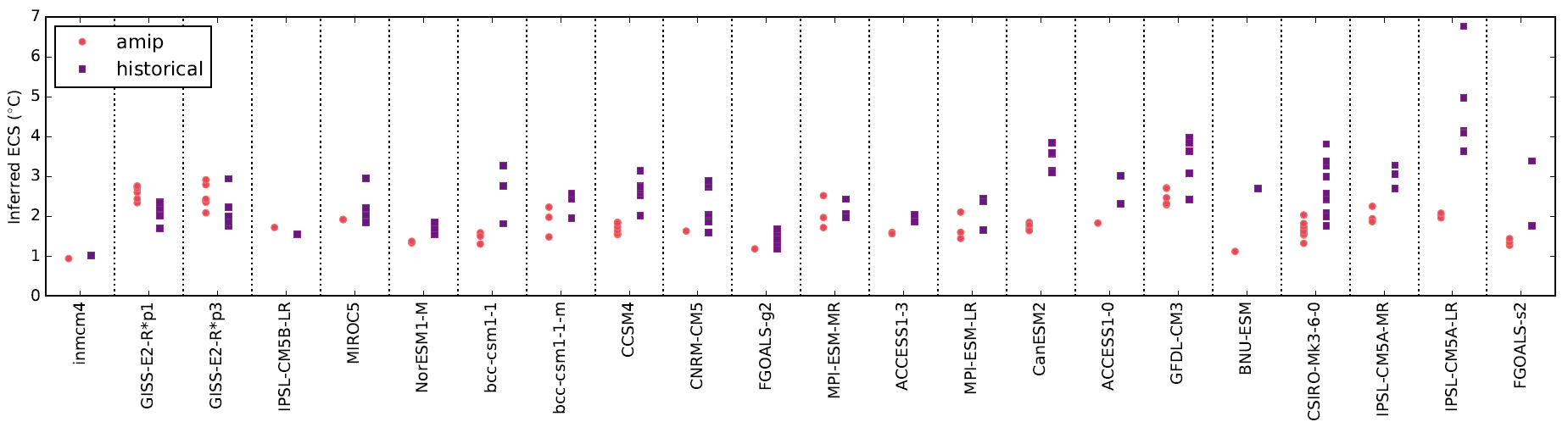
Figure 1. ECS estimated from recent (1979-2005) AMIP and historical simulations for each model’s ensemble of runs. Models are ordered by increasing estimated long-term ECS. Reproduced from Figure 1 of the Supporting Information for Marvel et al. (2018).
.
ECS estimates from historical simulations
The median ECS that Marvel et al. infer from1979-2005 historical simulation data is 2.3°C, significantly lower than the median long-term ECS estimate of 3.1°C.[12] However, there is an obvious possible explanation for these low ECS estimates from historical simulation data.
The 1979-2005 period is particularly unsuitable for ECS estimation since strong negative volcanic forcing arose during its first half, but not thereafter. There is evidence (including from Marvel et al.’s 2016 paper) that volcanic forcing has a low efficacy – it has much less effect on global temperature than the same CO2 forcing.2 [13] Accordingly, over the 1979-2005 period one would expect volcanism to increase the trend in F by a greater percentage than the trend in T, hence increasing the estimate of λ and depressing that of ECS.
It is simple enough to investigate the effect on short-period ECS estimation of avoiding significant influence from volcanism. I do so by using historical simulation data from the almost identical 1977-2005 period and Marvel et al.’s alternative decadal changes ECS estimation method. I made up the base ten years by combining the volcanic-free 1977-1981 and 1986-1990 periods. I took average changes from the base ten years to the final decade, 1996-2005, which is also free of eruptions. Doing so avoided the 1982 El Chichon and 1991 Mount Pinatubo eruptions and the main parts of the recoveries from each of them.
Figure 2 shows the resulting ECS estimates, upon applying equation (1).[14] The ECS estimates from individual simulation runs (red circles) are all over the place, as one would expect when estimating ECS from changes taking place over an average period of under twenty years. The change ΔF in average ERF is only 0.7 Wm−2, so in the odd run where a model exhibits large positive internal variability in ΔN between the split base period and 1996-2005 the denominator in (1) will be small, and thus the ECS estimate very high. In a modern observationally-based ECS estimate the ΔF value would typically be three times as large.
Where several historical simulation runs were carried out by a model, the ECS estimates using mean values from its ensemble of runs (red triangles) are less wild. But the interesting point shown in Figure 2 is that, across all models, the median of the long-term ECS estimates (blue line: 3.29°C) is almost identical to the median of the model-ensemble means based ECS estimates (red line: 3.37°C).[15] So, when care is take to avoid volcanism distorting the estimates, it is not true that ECS inferred from the recent historical period is “almost uniformly lower than that inferred from simulations subject to abrupt increases in CO2 radiative forcing”, as claimed by Marvel at el.
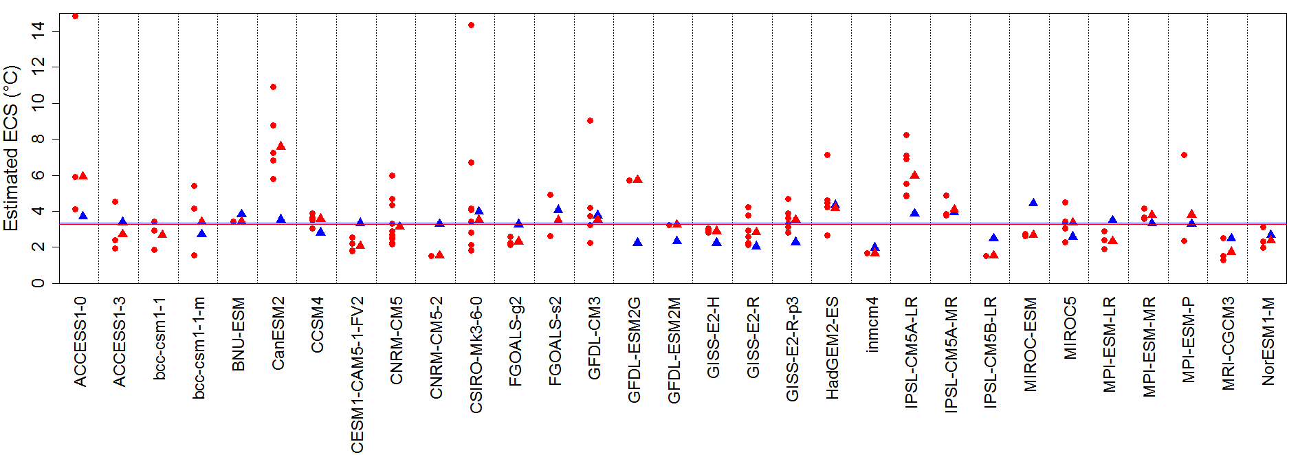
Figure 2. ECS estimated from non-volcanic periods in recent (1977-2005) historical simulations. Red triangles and circles show ECS estimated respectively from each model’s ensemble-mean values and from individual runs. Blue triangles show estimated long-term ECS. The red and blue lines (which overlap) show the multimodel-ensemble medians of respectively ensemble-mean ECS estimates and long-term ECS estimates. Long-term ECS was estimated using the same method as Marvel et al.
.
It is not possible to find a long period in historical simulations that avoids both significant volcanic activity and a large change in aerosol forcing. However, it is possible to improve the estimation of CMIP5 model ECS values by extending the period forward to 2016, splicing on data from RCP8.5 simulation runs that continue historical simulation runs after 2005, so as to use a final period of 2007-2016, as before taking changes relative to the combined 1977-81 and 1986-1990 periods.[16] The median within-model standard deviation of the resulting ECS estimates based on single simulation runs is then 13% of the median ensemble-mean ECS estimate. If that is taken as a proxy for the effect of internal variability on ECS estimation, it is not too bad given that this estimate is based only on data spanning a thirty year period, and on averaging over single decades.
For observationally-based energy-balance climate sensitivity estimation, where concern about model aerosol ERF strength is not a concern, one would normally use a much earlier (and typically rather longer) base period, thereby achieving a higher signal-to-noise ratio. If the full historical period to date is used to estimate model ECS values from simulation data, better precision is achievable. When using changes between the means for 1859-1882 and 1995-2016, two volcanism free periods, the median single-run ECS estimate standard deviation is only 8% of the median ensemble-mean ECS estimate. On that basis, uncertainty in observationally-based ECS estimation arising from internal variability is minor compared with other uncertainties.
ECS estimates from AMIP simulations
Marvel et al.’s median ECS estimate from CMIP5 AMIP simulations (1.8°C) was lower than that from historical simulations. A similar finding was shown (with volcanic years excluded) in Tim Andrews’ Ringberg talk in March 2015, and Gregory and Andrews (2016) gave sensitivity estimates for all models with AMIP simulations, albeit without identifying them, as well as their average.[17] It appears that the observed evolution of SST gave rise to enhanced tropical low-cloud cover compared to that in CMIP5 models’ historical simulations. The AMIP runs, which generally span 1979-2008, are too short to tell one much about the underlying cause, but in this case I think the lower ECS estimates for models are probably primarily genuine, rather than artefacts arising from use of a period with unbalanced volcanism. This is a reflection of Marvel et al.’s argument (c), which I put to one side earlier.
Marvel et al. claim that the low ECS values when models are driven by the observed evolution of SST patterns suggests that the “specific realization of internal variability experienced in recent decades provides an unusually low estimate of ECS.” However, as they admit, this is based on the perfect-model framework, which assumes “that the models as a group provide realistic descriptions of the mechanisms underlying observed climate variability”.
An alternative explanation for the models as a group misestimating the actual temporal evolution of SST change patterns is that the models as a group are imperfect. To my mind that should be the null hypothesis, rather than that internal variability over the last few decades results in an unusually low estimate of ECS. Indeed, the fact that internal variability linked to the Atlantic multidecadal oscillation is thought to have boosted warming over 1979-2005[18] makes it seem even less likely that in the real climate system ECS estimates based on this period would be biased low. Moreover, internal variability sufficient to produce a 20-year excursion of the magnitude required to account for the CMIP5 model average difference in N between AMIP and historical simulations does not appear to occurred in any of the 13,000 odd overlapping 20 year segments of their preindustrial control simulations.
Even if CMIP5 models don’t do too bad a job of simulating atmospheric behaviour, it is entirely possible that the real ocean is better able to move heat around the Earth’s climate system, in a way that reduces average surface temperature, than CMIP5 model oceans are able to do in their simulated climate systems. Marvel et al. recognize this, saying that the low ECS estimates derived from AMIP simulations “could also arise from the failure of the coupled models to reproduce aspects of the forced response”. Moreover, it is not the case that low model ECS estimates when driven by observed evolving SST patterns are limited to the last few decades. For now I will refrain from further discussion of this interesting area, which is a focus of research activity, as this article is already overlong.
Nic Lewis February 2018
.
[1] The paper itself is pay-walled, but the Supporting Information is not.
[2] Marvel, K., Schmidt, G. A., Miller, R. L., & Nazarenko, L. S. (2016). Implications for climate sensitivity from the response to individual forcings. Nature Climate Change, 6(4), 386.
[3] They mention, as examples:
Gregory, J. M., R. J. Stouffer, S. C. B. Raper, P. A. Stott, and N. A. Rayner (2002), An Observationally Based Estimate of the Climate Sensitivity, J. Climate, 15 (22), 3117-3121;
Otto, A., F. E. Otto, O. Boucher, J. Church, G. Hegerl, P. M. Forster, N. P. Gillett, J. Gregory, G. C. Johnson, R. Knutti, et al. (2013), Energy budget constraints on climate response, Nature Geoscience, 6 (6), 415-416;
Lewis, N., and J. A. Curry (2015), The implications for climate sensitivity of AR5 forcing and heat uptake estimates, Climate Dynamics, 45, 1009-1023.
[4] In the outlier land use change forcing run by the GISS-E2-R model that they used, ocean convection appears to have partly collapsed in the North Atlantic, as it does in some of that model’s main CMIP5 simulations.
[5] Hansen, J. E. et al. Efficacy of climate forcings. J. Geophys. Res. 110, D18104 (2005).
[6] E. L. Davin, N. de Noblet-Ducoudre, and P. Friedlingstein (2007), Impact of land cover change on surface climate: Relevance of the radiative forcing concept. Geophys. Res Lett, 34, L13702.
[7] Armour, K. C., C. M. Bitz, and G. H. Roe (2013), Time-varying climate sensitivity from regional feedbacks, Journal of Climate, 26 (13), 4518-4534; Gregory, J. M., T. Andrews, and P. Good (2015), The inconstancy of the transient climate response parameter under increasing CO2, Philos. Trans. R. Soc. London. (Described by Marvel et al. as “in press” but in fact published in October 2015.)
[8] Byrne, B., and C. Goldblatt (2014): Radiative forcing at high concentrations of well‐mixed greenhouse gases. Geophys. Res. Lett., 41, 152–160, doi:10.1002/2013gl058456; and
Etminan, M., G. Myhre, E. J. Highwood, and K. P. Shine (2016): Radiative forcing of carbon dioxide, methane, and nitrous oxide: A significant revision of the methane radiative forcing. Geophys. Res. Lett. 43(24) doi:10.1002/2016GL071930.
[9] Since ECS is defined as the eventual temperature rise going from 1⤬ to 2⤬ (preindustrial) CO2 levels, and recent levels are approximately 1.4⤬ preindustrial. If feedbacks change with a perturbation of 4⤬ CO2, that would be a problem when using climate model simulations involving 4⤬ CO2 to estimate their ECS, as is typically done, but there is little model evidence of that being the case.
[10] See my analyses here and here. The best estimates of ECS for CMIP5 models are now generally obtained by scaling the x-intercept of a regression fit to years 21-150 of ΔT and ΔN data from a simulation in which a model’s CO2 concentration is abruptly quadrupled (‘abrupt4xCO2’), thus omitting the early decades in which higher feedback strength (lower sensitivity) is exhibited.
[11] They presumably estimated λ as the ratio of the inter-decade change in (ΔF− ΔN) to that in ΔT. This method is arguably more robust than using regression.
[12] Derived from scaling the x-intercept of a regression fit to years 1-150 of ΔT and ΔN simulation data after a model’s CO2 concentration is abruptly quadrupled. On average, this method appears to underestimate CMIP5 models’ ECS values, but only by 5-10% compared to estimates derived from the now generally preferred method of regressing over years 21-150.
[13] E.g., Gregory, J. M., Andrews, T., Good, P., Mauritsen, T., & Forster, P. M. (2016). Small global-mean cooling due to volcanic radiative forcing. Climate Dynamics, 47(12), 3979-3991.
[14] I derived ECS estimates for all models for which I could obtain data for their historical, preindustrial control and abrupt CO2 quadrupling experiments, using data from the latter two experiments to estimate a model’s long-term ECS.
[15] If 1977 and 1978 are excluded from the initial years, there is little change in the average ensemble-mean ECS estimate: the mean increases slightly and the median is marginally lower.
[16] I extended the AR5 forcing series from 2011 to 2016 using primarily observationally-based estimates. The resulting increase in anthropogenic ERF over that period was 0.23 Wm−2, the same as per the RCP8.5 forcings dataset.
[17] Gregory, J. M., and T. Andrews (2016), Variation in climate sensitivity and feedback parameters during the historical period, Geophys. Res. Lett, 43 (8), 3911-3920.
[18] E.g., DelSole, T., Tippett, M. K., & Shukla, J. (2011). A significant component of unforced multidecadal variability in the recent acceleration of global warming. Journal of Climate, 24(3), 909-926.


43 Comments
Well done Nic.
Thanks, Anthony!
They should run these papers by Nic, before they submit them to the journals. But they don’t care.
> “But they don’t care”
Nor do they need to if so disposed.
That goes without saying. Yet you felt compelled to say it.
Rather you seem compelled not to.
Nic has the right technique in my view – produce critiques for publication in accessible platforms such as this website that may reach many more people than pay-walled journals.
Hoping that the activists will suddenly become scrupulously honest in their public dealings is less likely than Stepping Through the Looking Glass with Alice.
Reblogged this on Green Living 4 Live.
Nic: This subject is getting massively complicated. Some comments on what I do understand:
1) AMIP runs give a low climate sensitivity that agrees with EBMs. I think this means that the outward flux of LWR in the model must be reasonable. Many say that the ocean must be behaving differently in historical runs exhibiting higher climate sensitivity. However, the downward flux of SWR and LWR into the oceans could also be wrong. The AMIP process would remove the extra heat from the oceans.
For example, if the model has too few boundary layer clouds, absorption of SWR by the ocean might show a large bias, but emission of LWR to space could show little bias.
2) The key issue seems to be: What is more reliable? A single “realization” of our planet’s climate (subject to unforced variability) or multiple realizations of model output from multiple models?
2a) How good are the models? We have multiple realization of seasonal warming that have been observed from space. Tsushima (2013) shows AOGCMs can’t simulate the feedbacks we observe from space during the 3.5 K seasonal cycle. Therefore, the models aren’t fit for the purpose for which they are being used. LWR cloud feedback observed from space during the seasonal cycle is slightly negative, while the multi-model mean is positive, making the models biased toward high ECS. The observed SWR response to seasonal warming is not linear with temperature (partially due to lags). It is probably poorly reproduced by models too.
2b) Climate sensitivity has been calculated using EBMs over periods of 40 years, 65 years, 130 years and four individual decades. They all produce similar central estimates. The suggestion that EBMs are wrong because of unforced variability seems insane.
Nick Stokes has a triangular “trend viewer” that shows by color the warming trend for every possible starting year to every possible finishing year. The importance of unforced variability is clearly obvious in these triangles. If it were possible to construct something similar for the TCR and ECS of EBMs, it might illustrate the unimportance (or importance) of unforced variability in EBMs. I don’t know if you have enough data for such a project.
Frank
Thanks for your thoughtful comment.
1) The AMIP process, by imposing different SST patterns, changes the extent and distribution of clouds. In particular, it seems to lead to higher tropical marine low cloud cover (LCC) compared with historical simulations (Marvel et al. Fig. 3(b) and 3(c): there are only three models in common but they all show a greater 1979-2005 LCC increase in AMIP than in historical simulations. Volcanism could have biased this comparison, but I imagine the sign of the difference is correct. So downwards flux into the oceans, and its counterpart downwards TOA radiative imbalance, would indeed become relatively lower in AMIP runs. Which is what happens in the CMIP5 average, almost entirely due to an increase in the amount of SW solar radiation being reflected, as one would expect from greater LCC.
2) Yes. I shall write something more on this in due course. I think the evidence favours the observational record, notwithstanding that it is a single realization of the planet’s climate.
2a) I agree.
Re a ‘trend viewer’, I wrote a note in late 2015 that showed how TCR estimates varied over many different starting and finishing decades. It is available here: https://niclewis.files.wordpress.com/2018/02/sensitivity-of-simple-model-tcr-estimates-to-analysis-period_dtmin0-3.pdf. Decadal resolution is preferable to annual IMO, as it greatly reduces the influence of interannual variability (ENSO etc.). Multidecadal variability (mainly AMO) does have some effect on estimation, but generally the estimates are remarkably similar across analysis periods. If ocean heat uptake efficiency (the ratio of heat uptake change to GMST change) is constant, which is thought to be a reasonable approximation over the historical period, then stability of TCR estimates implies stability of energy-balance ECS estimates.
Nic: Thanks for the kind reply. I looked at the chart you provided. TCR certainly looks reasonably consistent over various periods. I tried, but failed, to use it to see if TCR was the same over many different 65-year periods, but was different for longer or shorter periods.
I pictured looking at the data as in the link below. If you follow the faint diagonals rising 45 degrees up and to the right from the years 2000, 1980, 1960, 1940, and 1920, the change in colors shows the change in 100-, 80-, 60-, 40-, and 20-year warming trends. At the x-axis, these are warming trends starting in 1900 and on the y-axis these are warming trends ending in 2017.
https://moyhu.blogspot.com.au/p/temperature-trend-viewer.html
Warming trends for periods of 60 years and longer show a gradual steady increase since 1900 due to rising forcing. Warming trends of 40 years and shorter fluctuate due to unforced variability (and volcanos).
A table of ECS derived from EBMs over periods of 40?, 65, 90? and 130 years using different starting years would be easier and communicate the same message as Stoke’s triangle. (The advantage of the triangle is that one can click on it to get – or cherry-pick – data for any point.)
FWIW, I dislike the assumption that ocean heat uptake efficiency is constant. If unforced variability were a confounding factor, then I would expect ocean heat uptake efficiency to vary chaotically with ocean currents. However, if this efficiency doesn’t vary with time in AOGCMs then the assumption you use to convert TCR to ECS is equally problematic in both methods for assessing ECS.
It seems a stretch to postulate theorems about “warming trends 60 years and longer and warming trends 40 years and shorter” when the interval of study is only 117 years. This is too much like climate science.
Nic: Do to its importance, I reformulated my “which is more reliable” question below. Same idea; better explanation.
Consensus scientists assert that unforced variability in a “single realization” of observed climate COULD bias ECS estimates from EBMs. To address this problem, they offer ECS derived from multiple realizations from one or more models. Which is more reliable?
1) The feedbacks associated with seasonal warming in models are wrong. Therefore their ECSs are systematically unreliable, no matter how many realizations they provide.
2) Different periods provide different “realizations” of observed climate. The THEORETICAL issue posed by unforced variability is not significant IN PRACTICE for the central estimate of ECS from EBMs.
I’d say a stable TCR over different periods (and period lengths) also refutes the hypothesis that different forcing agents have markedly different forcing efficacies. The share of CO2 in total GHG forcing oscillated from about 50% to 80% (eg in the 2000s); if CO2 forcing had higher or lower efficacy than non-CO2 forcing you’d see the TCR estimate swinging up and down.
Nic,
I suspect you are never going to be Kate Marvel’s favorite person.
At least there is now tacit admission the models may be off in how they respond to forcing: “could also arise from the failure of the coupled models to reproduce aspects of the forced response”. I would count that as progress, even if meager.
they could have used this:
Source:
https://www.nature.com/articles/ngeo2098
Volcanic contribution to decadal changes in tropospheric temperature
Benjamin D. Santer, Céline Bonfils, Jeffrey F. Painter, Mark D. Zelinka, Carl Mears, Susan Solomon, Gavin A. Schmidt, John C. Fyfe, Jason N. S. Cole, Larissa Nazarenko, Karl E. Taylor & Frank J. Wentz
Nature Geoscience volume 7, pages 185–189 (2014)
doi:10.1038/ngeo2098
Figure 2 is very convincing.
Cross posted from Judith Curry’s blog:
Why this focus on ECS?
The concept of equilibrium CO2 levels is at odds with the peak oil scare and “Limits to growth”. You can’t bave both, so what is it?
We are observing a constant airborne fraction of CO2 which disproofs the dreaded sink saturation of the Bern model.
The necessary components for Catastrophic Anthropogenic Grobal Warming (CAGW) are:
1 An over the top emission scenario like RCP8.5;
2 Sink saturation which keeps this CO2 in the atmosphere;
3 A high value for climate sensitivity.
I would call this a science fiction horror scenario, not science, because all three components are highly unlikely.
Finally climate sensitivity has a very strong frequency component so climate models should study a pulse response of CO2 which is far more like the peak oil concept. Ramp and equilibruim forcing of climate models yield over the top TCR and ECS values which have no meaning in a pulse like CO2 emission.
The following low pass amplifier spectrum gives a more realistic picture of the frequency response for climate sensitivity, (note the resonance peaks!)
The geological evidence (looking at the entire Phanerozoic) indicates that natural sources of CO2 cannot [quite] keep up with sinks. Biological and other sources withdraw CO2 from circulation at a rate (presuming approximately constant supply) that depletes atmospheric CO2 to near lower limits. Once that lower boundary is reached planetary biology seems to bounce along teetering on the edge of a collapse. The Permian exhibits this and the Pleistocene parallels the Permian. Plant evolution seems to have become more efficient at carbon fixing over the Mesezoic and Cenozoic with the appearance of C4 and CAMS-cycle metabolisms (typical of grasses for instance and some flowering plants). These plant forms are adapted to carbon-supply and water-supply stresses. Grasses notably appeared only about 20 million years ago, indicating increasing evolutionary pressure on primary producers due to carbon supply shortfall.
See also the paper
The Frequency Response of Temperature and Precipitation in a Climate Model by Douglas G. MacMynowski,, Ho-Jeong Shin and Ken Caldeira
on the concept of frequency domain climate sensitivity
Click to access SP_GRLfrmt.pdf
RE: Don Monfort, “whatever . . . I’m out”
Any chance mpainter will join you?
Rubble, my sole comment on this thread is at Feb 6, 8:24 pm. That is where you should respond. Thanks.
This made me giggle…
“An emerging literature suggests that estimates of equilibrium climate sensitivity (ECS) derived from recent observations and energy balance models are biased low because models project more positive climate feedbacks in the far future.”
As someone who does software for a living in the context of continuous integration/unit-test frameworks, and with an advanced degree in numerical modelling, this is the silliest way to look at model validation *ever*.
The measured data don’t match the as yet unvalidated model… ergo the measurement must be wrong. Even better, it’s the part of the model (the far future projections) that is not only *unvalidated* but *impossible* to validate, as the data to validate it also live in that same far future.
As a good friend of mine would say, “that isn’t right, that isn’t even wrong.”
Yes, yes, and that particular fact has been repeated to the climate scientist/modeling confraternity one hundred thousand times over the past several decades without making the slightest impression in their thinking.
Ethically Civil: I agree with your comments about modelers. However, it is worth remembering that observations of our climate system are limited and (for the most part) made with equipment never intended to accurately measure changes on the order of 0.1 K/decade. The first high quality network of surface temperature stations was started in the US only about 2003. Integrating buoys into current SST measures produced a controversial change of 0.05 K in the 2000’s and the earlier mixture of buckets and engine intake measurements is an unresolvable mess. Satellites have been measuring bulk temperature of the atmosphere for almost 40 years, but UAH and RSS disagree by about 0.05 K/decade. Radiosondes were far worse. Our best atmospheric records -“re-analyses” – are the output of climate models constrained to agree with our observations. Ocean temperature below the surface was a huge mess before ARGO. Finally, the observed record is just a single “realization” of a chaotic climate system vulnerable to perturbation by one butterfly.
So, you should feel a little sympathy of a climate modeler who thinks his output provides a clearer picture of the real world than observation. This doesn’t excuse their failure to confront and resolve the discrepancies between models and observations, nor their lack of candor about the many problems with models when talking to policymakers and the public. Fortunately, they no longer are resisting the reality of a discrepancy between models and observations (EBMs).
It would be good to have a paper on climate recovery, based on sustainable conditions.
The concept of “climate recovery” is an anthropomorphism. Had the industrial revolution adding CO2 never occurred the Earth’s climate would see snows increasingly not melting through the summer at lower and lower latitudes. A vicious cooling spiral would have produced the inevitable resumption of the 90% dominant climate state of the Quaternary Period, glaciation. Indeed, modern civilization only arose due to a ~10,000-year reprieve in a 120,000-year cycle. Polar ice cores, both NH and SH, clearly show the Garden of Eden is actually hellish.
You assume all warming since the LIA to be all AGW without any contribution of natural variability. Although this assumption forms the core belief of AGW proponents, it has only a flimsy theoretical basis and is unsustainable otherwise, this theory being refuted by observations. The hypothesis that CO2 fluctuations is responsible Pleistocene climatic fluctuations has been refuted by ice cores.
You mean like this?
From the draft National Climate Assessment (2018):
“Global average temperature has increased by about 1.7°F from 1901 to 2016, and observational evidence does not support any credible natural explanations for this amount of warming.”
I do not assume all warming to be linear to AGW or the ice age fluctuations to be controlled by CO2. I assumed people know about natural variability and Milankovitch cycles if they come here.
“…and observational evidence does not support any credible natural explanations for this amount of warming.”
What they meant to say is that current model evidence in not credible to explain observed evidence. My favorite part of the National Climate Assessment (2018) is the claim that from AGW we should expect more extreme low temperatures as well as extreme highs. Following that Logic, if we kept on enhancing the greenhouse effect we would have the climate of the Moon.
Yes, DaveJR, a good example that is prima facie false: the endpoint of the time series is a super El Nino year, this high end point due exclusively to natural factors (ENSO). Your quote is typical AGW advocacy, a falsehood disguised as science.
DaveJR quoted the NCA: “Global average temperature has increased by about 1.7°F from 1901 to 2016, and observational evidence does not support any credible natural explanations for this amount of warming.”
The phrase “natural variability” is ambiguous. There is some evidence that variability due to solar and volcanic influences weren’t important to this warming (especially in the second half of the century), but that doesn’t address the possibility unforced (internal) variability. AFAIK, we don’t have a complete picture of how volcanos and solar activity could have caused the LIA or warm periods (MWP, RWP, etc) seen in ice core record. The highest estimate for negative solar forcing (TSI/4) during the Maunder minimum is -1 W/m2 and many are lower.
These assessments allows ignore all of what Schneider infamously called the “ifs, ands, buts and caveats” that distinguish ethical science from policy advocacy (“making the world a better place” through scary scenarios, simplified dramatic statements, and hiding doubts.) You’ve cited a simplified dramatic statement without caveats or doubts.
Those interested in learning more about natural variability of climate during the Holocene should start with the Holocene Pluvial, a period of extraordinary wetness during the early Holocene. This was when the Sahara was green and wet, as was the Gobi, western north America, and other regions presently arid. Pay no attention to any confused discursions on the question of whether climate varies naturally.
I guess time is a factor – we’ll just have to wait, to find out, from our observations.
Nic, have you seen James Annan’s criticism of your use of Bayesian priors, here?
It dates from 2014, and so may not be worth the bother. But comments are still open.
patfrank01, Yes, I saw James Annan’s criticism at the time, thanks. Essentially, he says that genuine prior information does exist in the radiocarbon dating case and that I should have used it. But the paper setting out the OxCal method that I was criticising stated “we should not include anything but the dating information”, which implies that it was intended NOT to use any prior information about the true date of an artefect. So James’ arguments are not relevant to my analysis. I tried to make this point, but he and his subjective Bayesian supporters ignored it.
Thanks for the reply, Nic. I didn’t like to think such criticisms should go unanswered.
The narrative always seems to take precedence, doesn’t it.
James Annan has criticized my work, too, but deleted my posts in defense.
Nic, (or anyone,)
Are you aware of any attempts to diagnose the AGW signal in any other way besides decadal-centennial trend in global Tavg? Has there ever been quantification of marine influence and a model or apriori algorithm to separating AGW from non-climate effects?
Ron: GMST (before anomalies are calculated) rises and falls 3.5 K every year. The feedbacks that are observed in response to this seasonal warming are large and easily measured by CERES: 2.2 W/m2/K and highly linear in the LWR channel. That is about +1 W/m2/K for combined WV+LR feedback and negigible LWR cloud feedback; an ECS of 1.8 K/doubling before SWR feedback.
However, seasonal warming (an average of 10 K of warming in the NH and 3K of cooling in the SH) is not global warming. There is a large amount of seasonal snow cover in the NH, but not the SH, which superficially looks like positive SWR feedback. The SWR isn’t very linear (lags warming?) and may not be relevant to global warming.
Climate model do a poor job of reproducing the feedback observed in response to seasonal warming, except LWR feedback through clear skies (Planck+WV+LR). Their cloud LWR feedback is biased positive. Their SWR feedbacks through clear and cloudy skies are wrong and mutually inconsistent.
Since the changes accompanying seasonal warming are large and reproducible, they definitively illuminate some, but not all aspects of climate sensitivity. See Tsushima and Manabe, PNAS (2013), freely accessible.
Frank, thanks and yes, I forgot about Ceres and satellite monitoring of radiation. What I was really thinking of was analysis of meteorological data.
Frank, has anyone looked at historical meteorological data for quantifying marine effect by region?
Nice work Nic.
“Even if CMIP5 models don’t do too bad a job of simulating atmospheric behaviour, it is entirely possible that the real ocean is better able to move heat around the Earth’s climate system, in a way that reduces average surface temperature, than CMIP5 model oceans are able to do in their simulated climate systems.”
I’ve pointed out before the “missing heat hiding in the oceans” argument probably doesn’t cut to the favor of higher ECS, since the hydrosphere is 1) 300x more massive than the atmosphere 2) barely changing average temperature since 1940, and 3) becoming cooler relative to the warming atmosphere since 1940. This is the kind of process for which the estimates can vary by orders of magnitude, but it’s usually a safe assumption the 2nd Law applies on some timescale of interest (i.e. the warmer the atmosphere gets, the more the balance shifts — a negative feedback).
2 Trackbacks
[…] https://climateaudit.org/2018/02/05/marvel-et-al-s-new-paper-on-estimating-climate-sensitivity-from-… […]
[…] https://climateaudit.org/2018/02/05/marvel-et-al-s-new-paper-on-estimating-climate-sensitivity-from-… […]