The four constraints that Caldwell assessed as credible
A guest post by Nic Lewis
In Part 1 of this article the nature and validity of emergent constraints[i] on equilibrium climate sensitivity (ECS) in GCMs were discussed, drawing mainly on the analysis and assessment of 19 such constraints in Caldwell et al (2018; henceforth Caldwell),[ii] who concluded that only four of them were credible. All those four constraints favoured ECS in the upper half of the CMIP5 range (3.4–4.7°C). An extract of the rows of Table 1 of Part 1 detailing those four emergent constraints is given below.[iii]
| Name of constraint | Year | Correlation in CMIP5 | Description |
| Sherwood D | 2014 | 0.40 | Strength of resolved-scale mixing between BL and lower troposphere in tropical E Pacific and Atlantic |
| Brient Shal | 2015 | 0.38 | Fraction of tropical clouds with tops below 850 mb whose tops are also below 950 mb |
| Zhai | 2015 | –0.73 | Seasonal response of BL cloud amount to SST variations in oceanic subsidence regions between 20-40°latitude |
| Brient Alb | 2016 | –0.71 | Sensitivity of cloud albedo in tropical oceanic low-cloud regions to present-day SST variations |
Caldwell regarded a proposed emergent constraint as not credible if it lacks an identifiable physical mechanism; is not robust to change of model ensemble; or if its correlation with ECS is not due to its proposed physical mechanism. The credible constraints identified in Caldwell are all related to tropical/subtropical low clouds and all except Brient Shal are significantly correlated with each other.
Figure 1 shows the geographical distribution of the dominant sources of correlation for each of the emergent constraints assessed as credible. In each case the principal source is cloud feedback, dominantly shortwave (SW). The spatial pattern of correlation between the emergent constraint and ECS arising from cloud feedback is strikingly similar for all four constraints, despite their metrics being based on differing regions. Inter-model variation in forcing for a doubling of CO2 also has a non-negligible contribution for two of the four constraints. Other feedbacks account for that part of the total correlation not attributable to cloud feedback and 2⤬ CO2 forcing, and in aggregate are small except for Brient Shal.[iv]
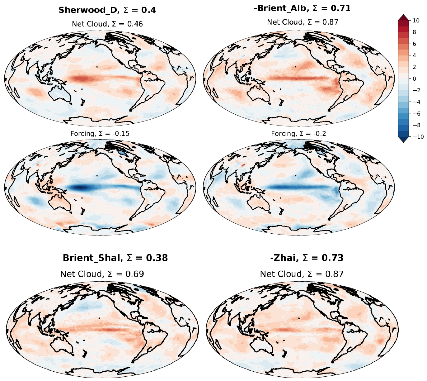
.
Of the studies proposing the four emergent constraints that pass Caldwell’s tests, Sherwood et al. has over four times as many citations (313) as the other three studies between them, so I will start by examining the validity of its emergent constraints. They are also discussed in an informative earlier review of emergent constraints, Klein and Hall (2015),[v] which (unlike the Caldwell paper) is open-access.
Sherwood
Sherwood et al. summed two physically-based metrics, D and S, to form a lower-tropospheric mixing index (LTMI) and used that as their principal emergent constraint. Caldwell found that while Sherwood S is meant to operate through SW cloud feedback, in CMIP5 models it actually gains correlation almost entirely through other terms. They therefore assessed both Sherwood S and Sherwood LTMI as not being credible.
However, Caldwell assessed Sherwood D, which predicts tropical low cloud changes due to boundary layer (BL) drying by convection, as credible. Nevertheless, while Sherwood D is computed using data from the tropical Atlantic and East Pacific, Caldwell found that its correlation with cloud feedback there is smaller than in the West Pacific (see top LH panel of Figure 1). That might cast doubt on the credibility of D, since its physical mechanism was predicted to occur over cooler oceans where mid-level outflows of ascending air occur, rather than in warm tropical oceans such as the West Pacific where such outflows do not usually occur. [vi] Moreover, Brient et al. (2015) found that while the convective mixing strength mechanism proposed by Sherwood et al. occurs in all GCMs, it only controls the low cloud response in about half the CMIP5 models.
Zhao et al (2016)[vii] showed that when they varied the convective precipitation parameterization in the new GFDL AM4 model, Sherwood LTMI and D changed little, and non-monotonically, between their high, medium and low ECS model variants. They say “It is clear that the two low-sensitivity models (M and L) produce a larger increase in upward water flux near the top of the boundary layer (800–900 hPa) than the high-sensitivity model (H)”, which is the opposite of the fundamental physical mechanism posited in Sherwood et al., being “that an increase of upward transport of moisture near the top of the boundary layer over the convective regions should result in decrease of low clouds because of dehydration of the boundary layer”.
If one takes Sherwood D at face value, all CMIP3 models and all but two CMIP5 models (ACCESS1-3 and CSIRO-Mk3-6-0) are unsatisfactory, in that they are inconsistent with the reanalysis-based estimates of D. Alternatively, if the reanalysis values are contaminated by model biases and a majority of models are actually consistent with the true value of D, then the Sherwood D constraint would not rule out low sensitivity models. In addition to this problem, the Sherwood D constraint seems to lack robustness to changes in the ensemble of models. Caldwell noted that Kamae et al. (2016)[viii] found that Sherwood LTMI explained low cloud feedback but not ECS in a perturbed physics ensemble (PPE), suggesting a lack of robustness. Of direct relevance to Sherwood D, Kamae et al. find no clear relationship between D and ECS in their multiple model-variant PPE.[ix] Figure 2 compares the relationship between D and ECS found by Sherwood et al. with that found by Kamae et al. in two subsets of their 8-model variant PPE, being those model-variants with respectively old and new convection schemes (OldCnv and NewCnv).
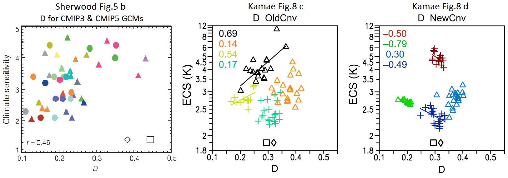
While only two of the models that Sherwood studied (both with higher than average ECS) have D values that are consistent with the reanalysis-based values, three of Kamae’s model-variants have, for some parameter values, D values consistent with the reanalysis-derived values. These D-value consistent cases have widely varying ECS values, many of them being between 2.1°C and 3°C. Moreover, the sign of the relationship between D and ECS varies between the model variants, being positive for five and negative for three. If one were to add the Kamae data to Sherwood et al.’s data the implications for ECS of the Sherwood D constraint would be very different.
The doubt arising from the geographical source of much of the ECS correlation with the Sherwood D constraint arguably not being consistent with the proposed physical mechanism, the finding by Zhao et al. that that mechanism has the opposite effect on ECS across their three model-variants to that proposed in Sherwood et al., and the non-robustness of the correlation between the CMIP3/CMIP5 data and the Kamae data, all point to Sherwood D not actually being a credible emergent constraint. In any event, Sherwood D only explains 16% of the CMIP5 intermodel ECS variance, so it is a weak constraint.
Brient Shallowness
Brient Shal is based on CMIP5 models with shallower tropical low clouds in weak-subsidence regimes tending to have a higher ECS. The paper’s authors did not view it as being about an emergent constraint, as they were fully aware of the limitations of climatological shallowness as an emergent constraint.(e.g., all models may misrepresent the relevant real-world dynamics in their parameterization schemes).[x] The point of the paper was that different models produce different low-cloud structures because of differences in the parameterizations; some of these differences in the present-day climatology correlate with the models’ response to warming. Brient et al. (2015) emphasised the importance of the competition between convective drying and turbulent moistening. They found that the climatological shallowness of low clouds was an indicator of the relative importance of parameterized convective and turbulent mixing in climate models, while the competition between these two mechanisms was a key determinant of the change in low cloud extent with surface warming and hence SW cloud feedback and ECS. These are interesting findings. However, the shallowness index has limited ability to discriminate between models with differing climate sensitivity. Brient et al. found that CMIP5 models that had shallowness indexes consistent with observational estimates had ECS values spanning almost the entire CMIP5 range. Brient Shal explains even less of the CMIP5 intermodel ECS variance than Sherwood D – only 14%. Moreover, its rather weak 0.38 correlation with ECS in CMIP5 models (it could not be tested on CMIP3 models) arises entirely from the inclusion of four models that fail Caldwell’s clear-sky linearity test. The correlation for the 17 models that pass that test is negligible – only 0.05. There is no contradiction between any of this and what Brient et al. say in their paper – they did not claim that the shallowness measure is useful as an emergent constraint.
.
I will examine the other two constraints that Caldwell considered credible, Brient Alb and Zhai, and set out conclusions, in Part 3 of this article.
Nic Lewis March 2018
[i] An emergent constraint on ECS is a quantitative measure of an aspect of GCMs’ behaviour (a metric) that is well correlated with ECS values in an ensemble of GCMs and can be compared with observations, enabling the derivation of a narrower (constrained) range of GCM ECS values that correspond to GCMs whose metrics are statistically-consistent with the observations.
[ii] Caldwell, P, M Zelinka and S Klein, 2018. Evaluating Emergent Constraints on Equilibrium Climate Sensitivity. J. Climate. doi:10.1175/JCLI-D-17-0631.1, in press.
[iii] The four studies involved are:
Brient, F., T. Schneider, Z. Tan, S. Bony, X. Qu, and A. Hall, 2015: Shallowness of tropical low clouds as a predictor of climate models’ response to warming. Climate Dynamics, 1–17, doi:10.1007/s00382-015-2846-0, URL http://dx.doi.org/10.1007/s00382-015-2846-0.
Brient, F., and T. Schneider, 2016: Constraints on climate sensitivity from space-based measurements of low-cloud reflection. Journal of Climate, 29 (16), 5821–5835, doi:10.1175/JCLI-D-15-0897.1, URL https://doi.org/10.1175/JCLI-D-15-0897.1.
Sherwood, S.C., Bony, S. and Dufresne, J.L., 2014. Spread in model climate sensitivity traced to atmospheric convective mixing. Nature, 505(7481), p.37-42.
Zhai, C., J. H. Jiang, and H. Su, 2015: Long-term cloud change imprinted in seasonal cloud variation: More evidence of high climate sensitivity. Geophysical Research Letters, 42 (20), 8729–8737, doi:10.1002/2015GL065911.
[iv] In Brient Shal the major contributors to the remaining correlation contribution of –0.23 are the residual error terms arising from model and equation non-linearity.
[v] Klein, S. A., & Hall, A., 2015. Emergent constraints for cloud feedbacks. Current Climate Change Reports, 1(4), 276-287.
[vi] Against that, Sherwood et al. argue that it is not expected nor required for the feedbacks to be concentrated in the same regions the constraints are measured.
[vii] Zhao, M., Golaz, J. C., Held, I. M., Ramaswamy, V., Lin, S. J., Ming, Y., … & Guo, H. (2016). Uncertainty in model climate sensitivity traced to representations of cumulus precipitation microphysics. Journal of Climate, 29(2), 543-560
[viii] Kamae, Y., Shiogama, H., Watanabe, M., Ogura, T., Yokohata, T., & Kimoto, M. (2016). Lower-tropospheric mixing as a constraint on cloud feedback in a multiparameter multiphysics ensemble. Journal of Climate, 29(17), 6259-6275.
[ix] The Kamie study involved creating 8 model variants with noticeably different key parameterization and closure schemes that affect cloud and convective behaviour, and then undertaking a PPE investigation for each. As a result of including 8 permutations of these structural model aspects they sampled a far wider range of model behaviour than a single-model PPE, which involves varying key parameters in a model but not structural aspects of it.
[x] Tapio Schneider, personal communication, 2018.


6 Comments
Nic, thanks for doing this. I read the conclusion as two of the four emergent constraints that Caldwell called credible, Sherwood D and Brient Shal, are actually not.
Off topic, I am wondering if you ever looked at the statistical validity of adjusting stations that move out of UHI or other non-climate effects. My thought is if one is studying a population (the stations) and there is random error of non-climate effects then there is no reason to make any adjustment. Just because a station typically becomes infected with non-climate effects gradually there is no reason that an individual’s local climate trend need be continuous in it’s trend. After all, the investigation is of the population of all land over many decades, not of each individual. So the only important aspect is that the population’s aggregate non-climate effects were measured in relatively the same in proportion to the actual climate signal near the beginning of the recorded time series as at the end.
Ron Graf, you have correctly summarized my conclusions in this article.
I’m afraid I haven’t looked at the issue you mention.
Thanks Nic. I always enjoy the education your posts bring.
Nic,
I look forward to your follow-up articles.
My starting prejudice is that the use of “emergent constraints” as a means of refining a predicted variable is fraught with epistemic problems. While Caldwell should be commended for recognizing SOME of the necessary conditions for credibility, he quite clearly does not have a complete list of necessary conditions, let alone a basis for sufficiency.
After trying (without success) to establish grounds for sufficiency, I checked back through several research engines to see where this methodology originated and where it has been applied before with proven success. The only references I can find to the use of “emergent constraints” apply to a quite different class of problem – namely where (a) one is trying to establish the intersecting set of conditions under which an event or regime change may occur and (b) the governing equations are already validated within the initial governing regime (pre-change).
Tracking back through the references in the papers you mention leaves me no wiser, in that I cannot find any examples of this approach having been used in other industries. As far as I can tell, the methodology you discuss here seems to have been invented by climate science, and only ever applied to climate science. This may just reflect the inadequacy of my research, and I would be grateful if you, or any reader, could point me to a similar application elsewhere – i.e. refinement of a quantity predicted from an ensemble of numerical experiments by cross-referencing intermediate correlative(s) (of the quantity) to observational data of the correlative(s).
The more normal approach to model validation is eschewed by climate science – with good reason from the modelers’ perspective. The models fail the more conventional approaches to validation. This is generally excused on the grounds that even the physical observations are just one realization of a stochastic system. Mmm, well maybe, but I would attach a lot more credibility to the models if the spread of results left the observational data somewhere in the middle rather than an outlier of numerous output series. Knutti (2008) explained the lack of validation as follows:-
In the specific example of SW cloud feedback appearing as a key correlative with ECS, we should not be surprised. Equally, we should not be surprised that the GCMs with high positive cloud feedback better match TOA SW change, since there was massive (poorly matched) SW heating over the satellite period and particularly between 1979 and the turn of the century. The two facts together however do not imply that the GCMs with high cloud feedback/high ECS yield a better value of ECS. (Although the conclusion would have a lot more credibility if there was a GCM which could simultaneously match the fields of cloud fraction, TOA LW, TOA SW, surface temperature and ocean heating!!!) The unstated assumption is that the physics of the GCMs are complete. A far more credible explanation is that the SW heating coincident with a large decrease in cloud albedo over this period was not a simple feedback to GHG-induced temperature change, but was in some significant part due to the quasi 60 year oscillation in climate indices, the mechanism for which remains elusive. Indeed, one of the major controls on clouds in the tropical region is ENSO which correlates to wind systems which correlates to AAM which is not matched on a long period basis (>7 years) by ANY of the AOGCMs.
I will save further ramblings for your follow-up articles.
I suspect the usage has derived from the area of emergent models of complex systems, of which GCMs are an example. There the realism of the emergent properties will influence the selection of constraints to reduce the solution set as part of model development. Validation would follow.
In this case those GCMs that weren’t doing a good job would be discounted. The problem as we know is that the implied ECS constraint is just one dimension of realism to be tested, so this means compromises in modelling constraints, and with that greater uncertainty over the GCMs’ output.
As you note the break with the emergent modelling community occurred when the frame of reference was shifted to earth simply being one realisation in what is no longer a ‘solution set’. In term of your quote I have never understood why the modelling community aren’t required to develop their models only using data up to 1950 (say).
Anyway I’ve wandered well off-topic which is simply whether accepting the current paradigm ECS can be constrained using these measures.
Paul,
Thank you for your thoughtful comment. I should perhaps have given a reference in Part 1 to the earliest use of an emergent constraint in climate science that I am aware of: Hall and Qu (2006): Using the current seasonal cycle to constrain snow albedo feedback in future climate change (open access).
I am not aware either of the emergent constraint approach being used outside climate science. I somewhat doubt that large ensembles of sophisticated numerical simulation models, all carrying out near-identical sets of simulations, and with only poor observational data available, even exist outside climate science.
I agree with what you say about multidecadal internal variability (in particular, the AMO) being a likely significant contributor to SW heating from the late 1970s to the early 2000s. However, if defence of the emergent constraint approach, most of them seem to depend on the response of the climate system to seasonal or interannual variability, not to multidecadal changes. Nevertheless, as you say, the major source of interannual variations, ENSO, is not independent of long period internal variability. I also worry about the differential impact of volcanism on the modelled and observed climate system behaviour distorting their comparison, in cases where either or both of the model simulations and observations used span a period that includes volcanic eruptions.
4 Trackbacks
[…] https://climateaudit.org/2018/03/23/emergent-constraints-on-climate-sensitivity-in-global-climate-mo… […]
[…] https://climateaudit.org/2018/03/23/emergent-constraints-on-climate-sensitivity-in-global-climate-mo… […]
[…] of the those four constraints, Sherwood D and Brient Shal, were analysed in Part 2 and found wanting. In this final part of the article I discuss the remaining two potentially […]
[…] of the those four constraints, Sherwood D and Brient Shal, were analysed in Part 2 and found wanting. In this final part of the article I discuss the remaining two potentially […]