A guest post by Nic Lewis
Judith Curry and I have now updated the LC15 paper with a new paper that has been published in the Journal of Climate
There has been considerable scientific investigation of the magnitude of the warming of Earth’s climate by changes in atmospheric carbon dioxide (CO2) concentration. Two standard metrics summarize the sensitivity of global surface temperature to an externally imposed radiative forcing. Equilibrium climate sensitivity (ECS) represents the equilibrium change in surface temperature to a doubling of atmospheric CO2 concentration. Transient climate response (TCR), a shorter-term measure over 70 years, represents warming at the time CO2 concentration has doubled when it is increased by 1% a year.
For over thirty years, climate scientists have presented a likely range for ECS that has hardly changed. The ECS range 1.5−4.5 K in 1979 (Charney 1979) is unchanged in the 2013 Fifth Assessment Scientific Report (AR5) from the Intergovernmental Panel on Climate Change (IPCC). AR5 did not provide a best estimate value for ECS, stating (Summary for Policymakers D.2): “No best estimate for equilibrium climate sensitivity can now be given because of a lack of agreement on values across assessed lines of evidence”.
At the heart of the difficulty surrounding the values of ECS and TCR is the substantial difference between values derived from climate models versus values derived from changes over the historical instrumental data record using energy budget models. The median ECS given in AR5 for current generation (CMIP5) atmosphere-ocean global climate models (AOGCMs) was 3.2 K, versus 2.0 K for the median values from historical-period energy budget based studies cited by AR5.
Subsequently Lewis and Curry (2015; hereafter LC15)[i] derived, using observationally-based energy budget methodology, a median ECS estimate of 1.6 K from AR5’s global forcing and heat content estimate time series, which made the discrepancy with ECS values derived from AOGCMs even larger. LC15 also derived a median TCR value of 1.3 K, well below the 1.8 K median TCR for CMIP5 models in AR5.
The LC15 analysis used a global energy budget model that relates ECS and TCR to changes (Δ) in global mean surface temperature [T], effective radiative forcing (ERF) [F] and the planetary radiative imbalance [N] (estimated from its counterpart, the rate of climate system heat uptake)[ii] between a base and a final period. The resulting estimates were considerably less dependent on comprehensive global climate models (GCMs) and allowed more thoroughly for forcing uncertainties than many others.[iii] Further information on the energy budget model is given in the Appendix to this article.
Considerable effort has been expended recently in attempts to reconcile observationally-based ECS values with values determined using climate models. Most of these efforts have focused on arguments that the methodologies used in the energy budget model determinations result in downwards-biased ECS and/or TCR estimates (e.g., Marvel et al. 2016; Richardson et al. 2016; Armour 2017).
We have now updated the LC15 paper with a new paper that has been published in the Journal of Climate “The impact of recent forcing and ocean heat uptake data on estimates of climate sensitivity“.[iv] The paper (hereafter, LC18) addresses a range of concerns that have been raised about climate sensitivity estimates derived using energy balance models. We provide estimates of ECS and TCR based on a globally-complete infilled version of the HadCRUT4 surface temperature dataset as well as estimates based on HadCRUT4 itself.[v] Table 1 gives the ECS and TCR estimates for the four base period – final period combinations used.
|
Base period |
Final period |
ECS |
ECS |
ECS |
TCR |
TCR |
TCR |
|
1869–1882 |
2007–2016 |
1.50 1.66 |
1.2–1.95 1.35–2.15 |
1.05–2.45 1.15–2.7 |
1.20 1.33 |
1.0–1.45 1.1–1.60 |
0.9–1.7 1.0–1.9 |
|
1869–1882 |
1995–2016 |
1.56 1.69 |
1.2–2.1 1.35–2.25 |
1.05–2.75 1.15–3.0 |
1.22 1.32 |
1.0–1.5 1.1–1.65 |
0.85–1.85 0.95–2.0 |
|
1850–1900 |
1980–2016 |
1.54 1.67 |
1.2–2.15 1.3–2.3 |
1.0–2.95 1.1–3.2 |
1.23 1.33 |
1.0–1.6 1.05–1.7 |
0.85–1.95 0.9–2.15 |
|
1930–1950 |
2007–2016 |
1.56 1.65 |
1.2–2.15 1.25–2.3 |
1.0–3.0 1.05–3.15 |
1.20 1.27 |
0.95–1.5 1.05–1.6 |
0.85–1.85 0.9–1.95 |
Lewis and Curry (2015) results for comparison |
|||||||
| 1859–1882 | 1995–2011 | 1.64 | 1.25–2.45 | 1.05–4.05 | 1.33 | 1.05–1.8 | 0.90–2.5 |
| 1850–1900 | 1987–2011 | 1.67 | 1.25–2.6 | 1.0–4.75 | 1.31 | 1.0–1.8 | 0.85–2.55 |
IPCC (2014) estimates for comparison |
|||||||
| AR5 (Chapter 12) | NA | 1.5–4.5 | 1–NA | NA | 1–2.5 | NA–3 | |
The new LC18 ECS and TCR estimates are very similar for all the period combinations used. That implies that the ‘hiatus’ – the period of slow warming from the early 2000s until a few years ago – had little effect on estimation. The preferred pairing is of the 1869–1882 and 2007–2016 periods, which provides the largest change in forcing and hence the narrowest uncertainty ranges, notwithstanding that both these periods are the shortest ones used. Using 1869–1882 as the base period avoids both any significant volcanism and the period of particularly sparse temperature data spanning most of the 1860s. Estimates are almost identical when using the longer 1850–1882 base period and excluding years affected by volcanism or with very sparse temperature data.
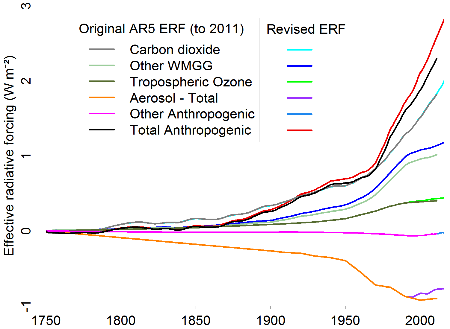
The new LC18 ECS and TCR HadCRUT4-based best estimates, respectively 1.50°C and 1.20°C, are approximately 10% lower than those in LC15. These reductions stem primarily from a significant upwards revision in estimated methane forcing following more accurate determination of the forcing-concentration relationships for the principal well-mixed greenhouse gases (WMGG)[vi] and revisions to post-1990 AR5 aerosol and ozone forcing estimates that reflect updated emission data,[vii] partially offset by a 2.5% upwards revision in the forcing from a doubling of preindustrial carbon dioxide (CO2) concentration, F2⤬CO2.[viii]
The 5% uncertainty bound of the AR5 2011 aerosol forcing estimate was changed from −1.9 Wm−2 to −1.7 Wm−2 to reflect substantial recent evidence against aerosol forcing being extremely strong.[ix] Doing so had virtually no effect on the median ECS and TCR estimates, and accounted for only a small fraction of the major reductions in their 83% and 95% upper uncertainty bounds from those in LC15. Most of that reduction is due to the revised forcing estimates and to average greenhouse gas concentrations over 2007–2016 being higher than over 1995–2011.
Figure 1 shows a comparison of the revised, extended forcings estimates with their original AR5 values. The significant increase in ‘Other WMGG’ forcing reflects the revision of the methane forcing component.[x]
There is some recent evidence that AR5 volcanic forcing estimates, which in LC18 are extended to 2016 using the AR5 calculation basis, may be biased low due to omission of volcanic aerosol in the lower stratosphere.[xi] However, once an adjustment is made for the background level of volcanic aerosol there appears to be virtually no effect on the changes in volcanic forcing between the base and final periods used in LC18.[xii]
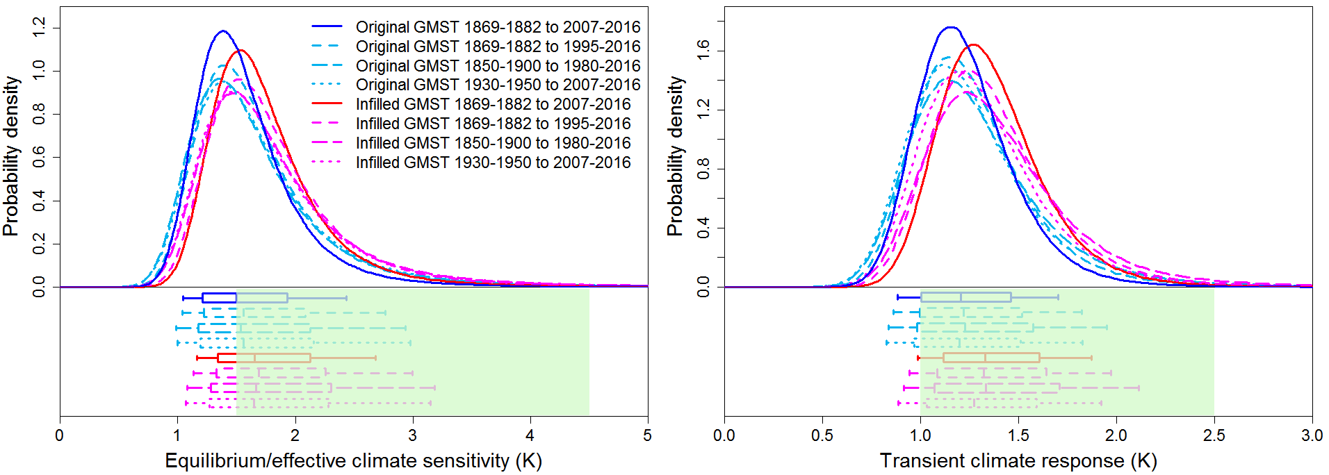
The new best estimates using globally-complete surface temperature data, of 1.66°C for ECS and 1.33°C for TCR, are almost the same as the LC15 ECS and TCR estimates based on non-infilled temperature data. Both the LC15 and LC18 ‘likely’ (66%+ probability) ranges are both very much towards the bottom ends of the corresponding IPCC AR5 ranges.
Figure 2 shows probability density functions for each of the ECS and TCR estimates, with the AR5 ‘likely’ ranges (shaded lime green) for comparison. The PDFs are skewed due principally to the dominant uncertainty in forcing, affecting the denominator of the fractions used to estimate ECS and TCR.
LC18 also derived, on comparable bases, ECS and TCR values for all current generation (CMIP5) GCMs for which the requisite data were available.[xiii] A majority of this ensemble of 31 CMIP5 models had ECS and TCR values that exceeded the 2.7°C and 1.9°C 95% uncertainty bounds that we derived for those parameters using globally-complete surface temperature data.
The foregoing ECS estimates reflect climate feedbacks over the historical period, assumed time-invariant. Two recent studies asserted that ECS estimates for CMIP5 models derived from forcing data comparable to that available for use in historical period (post-1850) observationally-based energy budget studies, using a constant feedbacks assumption, were biased low. They concluded that CMIP5 model ECS estimates were on average some 30% higher when derived from their response to an increase in CO2 concentration in a way that allows, insofar as practicable, for time-varying feedbacks.[xiv] We show that their calculations are biased and that, when calculated appropriately, the difference is under 10%.[xv] Allowing for such possible time-varying climate feedbacks increases the median ECS estimate to 1.76°C (5−95%: 1.2−3.1°C), using globally-complete temperature data. A majority of our ensemble of CMIP5 models have ECS values, estimated in the way designed to allow for time-varying feedbacks, that exceed 3.1°C.
It has been suggested in various studies that effects of non-unit forcing efficacy, temperature estimation issues and variability in sea-surface temperature change patterns likely lead to historical period energy budget estimates being biased low.[xvi] We examined all these issues in LC18 and found that only very minor bias was to be expected when using globally-complete temperature data.[xvii]
Over half of the 31 CMIP5 models have ECS values estimated using a comparable change in forcing to that over the historical period[xviii] of 2.9 K or higher, exceeding by over 7% our 2.7 K observationally-based 95% uncertainty bound using infilled temperature data. Moreover, a majority of these models have a TCR above our corresponding 1.9 K 95% bound.
The implications of our results are that high estimates of ECS and TCR derived from a majority of CMIP5 climate models are inconsistent (at a 95% confidence level) with observed warming during the historical period. Moreover, our median ECS and TCR estimates using infilled temperature data imply multicentennial or multidecadal future warming under increasing forcing of only 55−70% of the mean warming simulated by CMIP5 models.
I hope to discuss in more depth in a subsequent article some of the material in LC18 and its Supporting Information that has been dealt with only very briefly here.
.
Appendix – Further details of the energy budget method
In the energy budget method, external global mean estimates – observationally based so far as practical – of all forcing and climate system heat uptake components, as well as of surface temperature, are used to compute the mean changes ΔF in total forcing, ΔN in total heat uptake (≡ radiative imbalance), and ΔT in surface temperature, between a base period and a final period. An estimate of the strength of climate feedbacks (the climate feedback parameter, λ) acting between the two periods is obtained as:
λ = (ΔF − ΔN) / ΔT
By extrapolating this equation to equilibrium (ΔN = 0) and scaling ΔF to represent the radiative forcing attributable to a doubling of atmospheric CO2 concentration, F2⤬CO2, one obtains equilibrium climate sensitivity (ECS) as:
ECS = F2⤬CO2 / λ
It is assumed here that all types of forcing have the same effect on global surface temperature, i.e. that they have the same ‘efficacy’.
Equilibrium climate sensitivity (ECS) may thus be estimated as:
ECS = F2⤬CO2 ΔT / (ΔF − ΔN)
As AR5 (Section 10.8.1) says, the simple model represented by this equation follows from conservation of energy. However, as the equation is based on transient, non-equilibrium, changes what it directly estimates is an ‘effective climate sensitivity’, termed ECShist in LC18 when estimated using the change in forcing over the historical period or a comparable change. In order to estimate equilibrium climate sensitivity, the method makes the assumption that the feedback parameter λ is independent of ΔF and ΔT and constant over time, implying that ECS ≡ ECShist. The behaviour of CMIP5 models supports the assumed non-dependence of λ on ΔF or ΔT, at least up to a quadrupling of preindustrial CO2 concentration and warming of up to 5°C, but in most cases CMIP5 models exhibit a decline in λ as the time since imposition of a forcing increases, implying that ECS > ECShist. The estimated ratio of ECS to ECShist in each CMIP5 model is used in LC18 to derive an adjusted ECS estimate that reflects possible time-varying climate feedbacks.[xix]
AR5 (Section 10.8.1) also points out that TCR may be estimated as:
TCR = F2⤬CO2 ΔT / ΔF
provided that the change in forcing takes place gradually over an approximately 70-year timescale, which it does for all the base and final period combinations used.
.
Nic Lewis April 2018
.
[i] Lewis, N., and J. A. Curry, 2015: The implications for climate sensitivity of AR5 forcing and heat uptake estimates. Climate Dynamics, 45(3-4), 1009-1023. Note: the paper was initially published online in 2014. An article about the paper and its results was posted here.
[ii] Total heat uptake by the Earth’s climate system, 90%+ in the ocean, necessarily equals the Earth’s top-of-atmosphere radiative imbalance, neglecting the tiny and near-constant geothermal heat flux (which has a negligible effect on ΔN).
[iii] Although none of the forcing estimates used are fully independent of GCMs, they do not appear to be materially affected by the ECS and TCR values of the GCMs involved. The early industrial heat uptake estimates used are GCM-derived and dependent on the GCM’s sensitivity, but they are small and a correction factor is applied to allow for the sensitivity of the GCM being higher than the energy budget derived sensitivity estimate.
[iv] Lewis, N. ,and J. Curry, 2018:The impact of recent forcing and ocean heat uptake data on estimates of climate sensitivity. J. Clim. JCLI-D-17-0667 A copy of the final submitted manuscript, reformatted for easier reading, is available at my personal webpages, here. The Supporting Information is available here.
[v] Cowtan, K., and R. G. Way, 2014: Coverage bias in the HadCRUT4 temperature series and its impact on recent temperature trends. Quart. J. Roy. Meteor. Soc., 140(683), 1935-1944 (update at http://www.webcitation.org/6t09bN8vM).
[vi] Etminan, M., G. Myhre, E. J. Highwood, and K. P. Shine, 2016: Radiative forcing of carbon dioxide, methane, and nitrous oxide: A significant revision of the methane radiative forcing. Geophys. Res. Lett. 43(24) doi:10.1002/2016GL071930.
[vii] Myhre, G., and Coauthors, 2017: Multi-model simulations of aerosol and ozone radiative forcing due to anthropogenic emission changes during the period 1990–2015. Atmos. Chemistry and Phys., 17(4), 2709-2720.
[viii] The almost identical proportional reduction in HadCRUT4-based ECS and TCR estimates between LC15 and the new study reflects the fact that heat uptake and forcing changes increased in similar proportions relative to the temperature change.
[ix] See extensive discussion in section 3a of LC18. Note that the (revised) 2011 AR5 aerosol forcing uncertainty range is – as for all the AR5 forcing uncertainty ranges – merely used, after dividing by its median, to estimate fractional uncertainty in the ERF best estimate time series, as revised.
[x] The reason why recent CO2 forcing is almost unchanged despite F2⤬CO2 being 2.5% higher is that the revised greenhouse gas forcing formulae embody a slightly faster than logarithmic increase in CO2 forcing with concentration.
[xi] Andersson, S. M., et al., 2015: Significant radiative impact of volcanic aerosol in the lowermost stratosphere. Nature communications, 6, 8692.
[xii] LC18 Supporting Information, S1
[xiii] We excluded FGOALS-g2 as its 1pctCO2 simulation results are abnormal and the p2 variants of GISS-E2-H and GISS-E2-R as their model physics is intermediate between the main (p1) and p3 physics versions. That left 31 CMIP5 models. See Table 2 in the Supporting Information for their calculated ECS and TCR values. Note that the reference to ECS calculated on a comparable basis (to our observational energy budget ECS estimates) is to the ECShist values in Table 2.
[xiv] Armour, K. C., 2017: Energy budget constraints on climate sensitivity in light of inconstant climate feedbacks. Nature Climate Change, 7, 331-335.
Proistosescu, C., and P. J. Huybers, 2017: Slow climate mode reconciles historical and model-based estimates of climate sensitivity. Science Advances, 3(7), e1602821.
[xv] Section 7f and Supporting Information S5.
[xvi] Marvel, K., G. A. Schmidt, R. L. Miller and L. S. Nazarenko, 2016: Implications for climate sensitivity from the response to individual forcings. Nature Climate Change, 6(4), 386-389.
Richardson, M., K. Cowtan, E. Hawkins, and M. B. Stolpe, 2016: Reconciled climate response estimates from climate models and the energy budget of Earth. Nature Climate Change, 6(10), 931-935.
Gregory, J. M., and T. Andrews, 2016: Variation in climate sensitivity and feedback parameters during the historical period. Geophys. Res. Lett., 43: 3911–3920.
[xvii] See sections 7a, 7c and 7e of LC18.
[xviii] Where types of ECS estimate are distinguished in LC18, this type is termed ECShist. Since forcing in CMIP5 models’ historical simulations is model-dependent and unknown, their ECShist is estimated (in LC18 and other studies) using data from their simulations driven by known changes in CO2, in such a way as to mimic the ECS estimates that would be derivable from their responses to representative historical forcing.
[xix] See the fourth from last paragraph of section 7f in LC18 for details, and section S4 of the LC18 Supporting Information for the calculation of ECShist and ECS values for CMIP5 models.


24 Comments
Solid work as always
Can you report the values if you use
1859–1882
As the base period. In your previous work you used this period.
1. Why the change?
2. What effect does this change have on your answers.
Hi Steven,
Are you expecting 1859 is significantly different than 1869?
OT, does Berkeley Earth have a consensus as to the cause of the huge dip in land temp around 1800-1815? I am thinking the Dalton solar minimum is the prime suspect. Also, has it brought any curiosity that the dip starts a steep recover ~1815 just when a once in a millenium volcano erupts, Tambora 1815?
Click to access global-land-TAVG-Trend.pdf
“Are you expecting 1859 is significantly different than 1869?”
A. I have zero expectations.
B. There was a change in the analysis approach
1. I expect the effects of that analytical choice to be DETAILED
if there is no difference, then there is no need to change it.
if there is a difference, then the argument needs to be made in QUANTITIVE
terms. When you look at the text, the reasoning is vague and subjective
and not quantitative.
C. If the previous period (1859-1882) was in fact tested before the change to 1869 was made
Then the result must be reported and the reasons for change should be made in a clear
and transparent way.
Thanks for the reply Steven. You are absolutely correct to scrutinize the choice. This is Climate Audit.
Steven,
See section 4 of the paper for an explanation of the change from 1859-82 to 1869-82. It is linked to exceptionally poor observational coverage during most of the 1860s., something that I had not thought about at the time of the previous study.
The sensitivity analysis in Table 4 of the paper shows that the main 1869-82 to 2007-16 HadCRUT4-based median ECS estimate of 1.50 K is unchanged if a base period of 1850-82, with years having very low observational coverage or significant volcanic influence excluded, is used instead. My notes, if I read them correctly, indicate that using the 1859-82 period (all years) would increase the estimate by 0.03 K, or 2%.
“niclewis
Posted Apr 24, 2018 at 10:18 AM | Permalink | Reply
Steven,
See section 4 of the paper for an explanation of the change from 1859-82 to 1869-82. It is linked to exceptionally poor observational coverage during most of the 1860s., something that I had not thought about at the time of the previous study.”
I read that section and found no numerical analysis to back up the assertions.
Look at the green line in Fig.3. Also at the green line in the 4th panel of Figure 6 of the HadCRUT4 paper, Morice et al 2012 doi:10.1029/2011JD017187. Total uncertainty was 30-40% higher over most of the 1860s than it was over 1869-82.
Steve,
The civil war would of led to a fair number of sites being compromised.
Nic, thanks for your continued climate work and particularly your outreach to us in the blog community.
Does your analysis agree with the majority of GCMs in assumption of radiative imbalance during your starting periods and ending periods? What are those figures?
Most GCMs start their Historical period simulations from equilibrium, so have zero radiative imbalance in 1850 or 1860. As Gregory et al 2013 doi:10.1002/grl.50339, showed, due to the existince of preindustrial volcanic forcing that is unrealistic and biases these GCM historical simulations. I used his results from GCMs simulations starting in AD 850, which reflect preindustrial volcanism, to derive radiative imbalance in the 2nd half of the 19th century. I scaled them down by 40% to reflect the higher GCM sensitivity than that estimated in the paper.
Most CMIP5 GCMs overestimate radiative imbalance in the 2000s, although the Fig. 9.17 in the published IPCC AR5 implied to the contrary. See AR5 WG1 Errata Figure 9.17; Version 17/04/2015 (or later).
Nic, thanks for your detailed reply. The reason I asked is because I noticed that the Little Ice Age is concluded with a double hit of the Dalton Minimum and 1815 Tambora eruption, the later did not even register any cooling dip on the BE Land Temperature chart I linked above. If that chart’s global coverage was sufficient to be indicative of GMST then one could conclude that there was such a positive radiative imbalance at 1815 that even the forcing of a once in millennium magnitude eruption could not dip temps more. If that was the case then as solar forcing recovered from the Dalton Minimum, and aerosols cleared from the 1815 eruption, by mid century one might expect a significantly positive imbalance existed. If I understand your reply that is what you and Gregory 2013 are putting forth. So if the GCMs assume radiative equilibrium in mid 19th century and overstate positive imbalance in the 21st century this would explain a part of the discrepancy in ECS/TCR between observational based study versus AOGCM modeled.
Is that right?
Ron,
“So if the GCMs assume radiative equilibrium in mid 19th century and overstate positive imbalance in the 21st century this would explain a part of the discrepancy in ECS/TCR between observational based study versus AOGCM modeled.”
These factors certainly help explain why CMIP5 models do not on average overwarm during the historical period despite their high climate sensitivity, but forcing differences (particularly as to aerosol forcing) are probably a larger factor.
It seems the AOGCMs over-sensitivity to aerosols is a widely suspected factor but I never heard anyone else point to the models starting with a wrong assumption of radiative equilibrium. Of course, I’m sure I just missed it as obviously you were aware of it. I suppose the ~1.4C discrepancy in median ECS between LC18 and CMIP5 is just the combined effect of dozens of parameters, each guessed with the precautionary principle hanging overhead of concerned CMIP modelers.
There’s an article in the Express,
https://www.express.co.uk/news/uk/950748/climate-change-scientists-impact-not-as-bad-on-planet
Climate change is ‘not as bad as we thought’ say scientists
The study questioning the future intensity of climate change was carried out by American climatologist Judith Curry and UK mathematician Nick Lewis.
Pretty dumb article, IMHO. It keeps switching to the rising sea levels in Europe, as if that’s relevant.
Nic and Judith’s paper is actually making some headlines. Congrats to both.
https://www.investors.com/politics/editorials/global-warming-computer-models-co2-emissions/
Thanks for this analysis, Judith and Nic.
Your analysis assumes that all of the warming since 1869 was caused by greenhouse gases and that there has been no natural warming, and the HadCRUT4 temperature dataset is unaffected by the urban heat island effect (UHIE).
Earth climate history shows an obvious millennium temperature cycle as show by this graph of extra-tropical North America (ETNH)temperature proxies.

The temperature rise from 1869 to 1900 is all a natural recovery from the Little Ice Age (1400 to 1700) as humans could not have had any effect on climate during this period. The temperature rise from 1900 to 1950 is almost all natural, as the CO2 rise was insignificant. This shows that your assumption that the earth was in temperature equilibrium in 1869 – 1882 is false, and that a significant portion of the temperature rise was natural.
The global temperatures vary by only 80% of the ETNH according to HadCRUT4. The global natural recovery from the Little Ice Age since 1900 is estimated at 0.084 °C/century based on the millennium cycle from the graph and the global adjustment. This reduces the calculated equilibrium climate sensitivity (ECS) by 0.23 C.
Numerous papers have shown that the UHIE contaminates the instrument temperature record. A study by McKitrick and Michaels showed that almost half of the warming over land since 1980 in instrument data sets is due to the UHIE. A study by Laat and Maurellis came to identical conclusions. A study by Watts et al presented at the AGU fall meeting 2015 showed that bad siting of temperature stations has resulted in NOAA overestimating US warming trends by 59% since 1979. A study by Dr. Roy Spence also shows that about half the warming over land is UHIE. The UHIE over land is 0.14 °C/decade, or 0.042 °C/decade on a global basis since 1979. The UHIE
correction over the period 1980 to 2008 is 0.11 °C. Making the conservative assumption that there was no UHIE before 1980, this reduced the ECS by 0.20 C.
Correcting the Lewis & Curry ECS estimate for the preferred base and final periods, the ECS is reduced by 0.43 C from 1.50 C to 1.07 C.
Using the most recent version of the FUND integrated assessment model, assuming a 3% discount rate, emissions in 2018 and ECS = 1.50 C, the social cost (benefit) of carbon dioxide is +US$1.36/tonne CO2. However, using the corrected ECS of 1.08, the social cost (benefit) of carbon dioxide is US$-20.06/tonne CO2.
Using a more realistic discount rate of 5%, the SCC for 1.5 C and 1.08 C is US$-0.28/tonne CO2 and US$-10.61/tonne CO2, respectively. The negative signs means that the benefits of emissions exceeds the costs of emissions.
FUND is the world most detailed, evidence-based integrated assessment model.
Rather than imposing carbon taxes, fossil fuel use should be subsidized by US$10 to US$20/tonne CO2.
Ken, in fairness to Lewis and Curry (2018) their hands were tied to using assumptions that are either already in existing peer review literature or proved in their paper. I agree the official temperature indexes are biased but that is a separate fight.
For several years I thought the adjustments should be made to accurately reflect UHIE in the land record. Recently, I realized the illegitimacy of adjusting individual stations at all for anything but systematic changes in sensing adopted network-wide. Making adjustments in a statistical population to “fix” random error flies in the face of all statistical protocol. The consensus retort is that adjustments are necessary to restore homogeneity of station trend when they get relocated due to becoming unduly contaminated with non-climate effects, like UHIE. My answer is who cares if the individual trends are not smooth? The importance is only in the population’s trend. If a locality’s reporting is brought back to the uncontaminated state that it was originally reporting 100 years ago then the excursion in-between is just random error getting corrected. Hands off data!
When there is a change like the introduction of the Stevenson Screen sensor housing or a change in time of observation network-wide an adjustment is in order after rigorous concurrent side-by-side use of both methods for a 5-year overlap. If that was not done in the past it’s not too late to do. And how expensive would it be relative to global catastrophe or political imprudence?
Great stuff. I am surprised Gavin and his cohorts over at realclimate haven’t gotten right on this. /sarc
The Russia! Russia! bogeyman meme is still paramount amongst the 5 eyes & co: https://news.sky.com/story/mi5-boss-andrew-parker-accuses-russian-state-of-criminal-thuggery-11372257
Others like PR China or Gulf oil sheiks don’t exit apparently.
Wrong thread: please move..
Lewis & Curry slowly working toward the ‘unpublished’ conclusion of Monckton et al. (2018).
This site has a Canadian bent so here’s something from Canada that’s important:
Temperature and precipitation trends in Canada during the 20th century
Click to access Zhang%20Vincent%20Niitsoo%202000%20AO.pdf
“The annual mean temperature for Canada has increased by 0.3C over the last 49 years(1950-1998), but this increasing trend was not statistically significant.”
Authors however continue to believe in detrimental warming.
The great boil-off is happening before our eyes.
Global cooling is underway.
Come on Steve there’s work to be done . . .
Make ClimateAudit great again!
2 Trackbacks
[…] has a blog post about it at Climate Audit, and there’s also an article at GWPF, New data imply slower global […]
[…] In other words, the models predict way to much warming and do not match reality. More about the update here. […]