Jul 31, 2019: Noticed this as an unpublished draft from 2014. Not sure why I didn’t publish at the time. Neukom, lead author of PAGES (2019) was coauthor of Gergis’ papers.
One of the longest-standing Climate Audit controversies has been about the bias introduced into reconstructions that use ex post screening/correlation. In today’s post, I’ll report on a little noticed* Climategate-2 email in which a member of the paleoclimatology guild (though then junior) reported to other members of the guild that he had carried out simulations to test “the phenomenon that Macintyre has been going on about”, finding that the results from his simulations from white noise “clearly show a ‘hockey-stick’ trend”, a result that he described as “certainly worrying”. (*: WUWT article here h/t Brandon).
A more senior member of the guild dismissed the results out of hand: “Controversy about which bull caused mess not relevent.” Members of the guild have continued to merrily ex post screen to this day without cavil or caveat.
The bias, introduced by ex post screening of a large network of proxies by correlation against increasing temperatures, has been noticed and commented on (more or less independently) by myself, David Stockwell, Jeff Id, Lucia and Lubos Motl. It is trivial to demonstrate through simulations, as each of us has done in our own slightly different ways.
In my case, I had directed the criticism of ex post screening particularly at practices of D’Arrigo and Jacoby in their original studies: see, for example, one of the earliest Climate Audit posts (Feb 2005) where I wrote:
Jacoby and d’Arrigo [1989] states on page 44 that they sampled 36 northern boreal forest sites within the preceding decade, of which the ten “judged to provide the best record of temperature-influenced tree growth” were selected. No criteria for this judgement are described, and one presumes that they probably picked the 10 most hockey-stick shaped series. I have done simulations, which indicate that merely selecting the 10 most hockey stick shaped series from 36 red noise series and then averaging them will result in a hockey stick shaped composite, which is more so than the individual series.
The issue of cherry picking arose forcefully at the NAS Panel on paleoclimate reconstructions on March 2, 2006 when D’Arrigo told a surprised panel on March 2 that you had to pick cherries if you wanted to make “cherry pie”, an incident that I reported in a blog post a few days later on March 7 (after my return to Toronto.)
Ironically, on the same day, Rob Wilson, then an itinerant and very junior academic, wrote a thus far unnoticed CG2 email (4241. 2006-03-07) which reported on simulations that convincingly supported my concerns about ex post screening. Wilson’s email was addressed to most of the leading dendroclimatologists of the day: Ed Cook, Rosanne D’Arrigo, Gordon Jacoby, Jan Esper, Tim Osborn, Keith Briffa, Ulf Buentgen, David Frank, Brian Luckman and Emma Watson, as well as Philip Brohan of the Met Office. Wilson wrote:
Greetings All,
I thought you might be interested in these results. The wonderful thing about being paid properly (i. e. not by the hour) is that I have time to play.
The whole Macintyre issue got me thinking about over-fitting and the potential bias of screening against the target climate parameter. Therefore, I thought I’d play around with some randomly generated time-series and see if I could ‘reconstruct’ northern hemisphere temperatures.
I first generated 1000 random time-series in Excel – I did not try and approximate the persistence structure in tree-ring data. The autocorrelation therefore of the time-series was close to zero, although it did vary between each time-series. Playing around therefore with the AR persistent structure of these time-series would make a difference. However, as these series are generally random white noise processes, I thought this would be a conservative test of any potential bias.
I then screened the time-series against NH mean annual temperatures and retained those series that correlated at the 90% C. L. 48 series passed this screening process.
Using three different methods, I developed a NH temperature reconstruction from these data:
- simple mean of all 48 series after they had been normalised to their common period
- Stepwise multiple regression
- Principle component regression using a stepwise selection process.
The results are attached. Interestingly, the averaging method produced the best results, although for each method there is a linear trend in the model residuals – perhaps an end-effect problem of over-fitting.
The reconstructions clearly show a ‘hockey-stick’ trend. I guess this is precisely the phenomenon that Macintyre has been going on about. [SM bold]
It is certainly worrying, but I do not think that it is a problem so long as one screens against LOCAL temperature data and not large scale temperature where trend dominates the correlation. I guess this over-fitting issue will be relevant to studies that rely more on trend coherence rather than inter-annual coherence. It would be interesting to do a similar analysis against the NAO or PDO indices. However, I should work on other things.
Thought you’d might find it interesting though. comments welcome
Rob
Wilson’s sensible observations, which surely ought to have caused some reflection within the guild, were peremptorily dismissed about 15 minutes later by the more senior Ed Cook as nothing more than “which bull caused which mess”:
You are a masochist. Maybe Tom Melvin has it right: “Controversy about which bull caused mess not relevent. The possibility that the results in all cases were heap of dung has been missed by commentators.”
Cook’s summary and contemptuous dismissal seems to have persuaded the other correspondents and the issue receded from the consciousness of the dendroclimatology guild.
Looking back at the contemporary history, it is interesting to note that the issue of the “divergence problem” embroiled the dendro guild the following day (March 8) when Richard Alley, who had been in attendance on March 2, wrote to IPCC Coordinating Lead Author Overpeck “doubt[ing] that the NRC panel can now return any strong endorsement of the hockey stick, or of any other reconstruction of the last millennium”: see 1055. 2006-03-11 (embedded in which is Alley’s opening March 8 email to Overpeck). In a series of interesting emails (e.g. CG2 1983. 2006-03-08; 1336. 2006-03-09; 3234. 2006-03-10; 1055. 2006-03-11), Alley and others discussed the apparent concerns of the NAS panel about the divergence problem, e.g. Alley:
As I noted, my observations of the NRC committee members suggest rather strongly to me that they now have serious doubts about tree-rings as paleothermometers (and I do, too… at least until someone shows me why this divergence problem really doesn’t matter). —
In the end, after considerable pressure from paleoclimatologists, the NAS Panel more or less evaded the divergence problem (but that’s another story, discussed here from time to time.)
Notwithstanding Wilson’s “worry” about the results of his simulations, ex post screening continued to be standard practice within the paleoclimate guild. Ex post screening was used, for example, in the Mann et al (2008) CPS reconstruction. Ross and I commented on the bias in a comment published by PNAS in 2009 as follows:
Their CPS reconstruction screens proxies by calibration-period correlation, a procedure known to generate ‘‘hockey sticks’’ from red noise (4 – Stockwell, AIG News, 2006).
In their reply in PNAS, Mann et al dismissed the existence of ex post screening bias, claiming that we showed “unfamiliarity with the concept of screening regression/validation”:
McIntyre and McKitrick’s claim that the common procedure (6) of screening proxy data (used in some of our reconstructions) generates ”hockey sticks” is unsupported in peer reviewed literature and reflects an unfamiliarity with the concept of screening regression/validation.
CA readers will remember that the issue arose once again in Gergis et al 2012, who had claimed to have carried out detrended screening, but had not. CA readers will also recall that Mann and Schmidt both intervened in the fray, arguing in favor of ex post screening as a valid procedure.


101 Comments
The easiest people to fool were themselves.
===========================
Do not be fooled by the matador’s red cape.
good catch. I’ll note that up in text tomorrow. It’s a while since I looked at this material.
Steve,
My congratulations on your use of the non-judgmental term “guild”.
Keeping the tone of the descriptive narrative to neutral values can only
encourage rational discussion.
Stephen,
Can I post this on a new thread
\title{Analysis of Perturbed Climate Model Forcing Growth Rate}
\author{G L Browning}
\maketitle
Nick Stokes (on WUWT) has attacked Pat Frank’s article for using a linear growth in time of the change in temperature due to increased Green House Gas (GHG) forcing in the ensemble GCM runs. Here we use Stokes’ method of analysis and show that a linear increase in time is exactly what is to be expected.
1. Analysis
The original time dependent pde (climate model) for the (atmospheric) solution y(t) with normal forcing f(t) can be represented as
where y and f can be scalars or vectors and A coresspondingly a scalar or matrix. Now supose we instead solve the equation

where is the Green House Gas (GHG) perturbation of f. Then the equation for the difference (growth due to GHG)
  is
is

Multipy both sides by _{t} = \exp( A t ) \Delta f . Integrate both sides from 0 to t
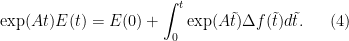
Assume the initial states are the same, i.e., is 0. Then multiplying by
  yields
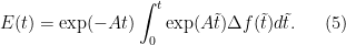
Taking norms of both sides the estimate for the growth of the perturbation is

where we have assumed the norm of as in the hyperbolic or diffusion case. Note that the difference is a linear growth rate in time of the climate model with extra CO2 just as indicated by Pat Frank.
Stephen,
I had to redo the last equation because latex2wp does not take macros.
Stephen,
Should be correspondingly. 😟
Also one equation missing. Will try to find out why.
Note this is the best estimate unless more is known about A as in the Bounded Derivative Theory.
Jerry
Am I misreading this? Surely the comment made by Ed Cook means they are all BS – but nobody noticed.
“Controversy about which bull caused mess not relevent. The possibility that the results in all cases were heap of dung has been missed by commentators.”
Read that the same way….
I also read it that way
Cook is indeed calling the reconstructions “BS.”
Cook became disaffected with Michael Mann’s bullying, and the result was a shot across the bow:
https://agupubs.onlinelibrary.wiley.com/doi/full/10.1029/2001GL014580
Even though Cook never bought into the smoothing-out of the MWP, he brusquely dismissed Steve’s request for data, so Steve has been on the attack ever since.
Indeed, Cook seems only able to criticize the consensus in private. In public he’s a staunch defender.
My thought on that comment, too. They don’t really believe what they publish. They just publish what brings in the dough.
Plenty of us noticed this, and there was a flurry of comments at the time. The trouble was the acceptance by so many that ad hominem attacks, a la Cook’s, were a normal and apparently acceptable part of scientific debate. The reality is that any time you see the debate turn from substantive issues to personalities, the party that initiated the “personalities” attack has evidently run out of evidence to support their view. They’ve given an “I’m right and this why …” style for “bulls make messes,” which says effectively nothing.
I don’t really want to beat on Rob:
“It is certainly worrying, but I do not think that it is a problem so long as one screens against LOCAL temperature data and not large scale temperature where trend dominates the correlation.”
I have no idea why he would automatically conclude that local temperatures would resolve the issue. Any admission by a scientist that the tree ring data contained even a small signal from non-temperature influences (and there is a lot of poorly correlated data) results in the over-selection of the favorable portion of the non-temperature signal and rejection of the unfavorable portion. This hand waiving argument is non-trivial and unscientific.
Tree ring growth may respond to factors other than temperature, such as rainfall, rainfall timing, cloud cover %, soil type and nutrient availability, plant disease, human activity, changes in atmospheric carbon levels and changes in other gases, air pressure, winds, tree site location (shading effects, etc), avalanches, to name a few.
Oh they truly do. The noise in the data is tremendous which is why the field has replaced what should have been simple data averaging methods with preferential data sorting. I wish all science worked like that because we could get so much more done!! All drugs would work, stocks would soar, anything we wanted could be done.
I have seen this described in the skeptic literature as “CO2 fertilization”.
Sorry for the obscure comment–by “this”, I mean the reference, above, to atmospheric carbon as a confounding factor in the interpretation of tree-ring data. Things grow faster when there is more CO2, I am told.
Jeff Id writes “Any admission by a scientist that the tree ring data contained even a small signal from non-temperature influences (and there is a lot of poorly correlated data) results in the over-selection of the favorable portion of the non-temperature signal and rejection of the unfavorable portion.”
regarding: “Controversy about which bull caused mess not relevent. The possibility that the results in all cases were heap of dung has been missed by commentators.”
No it wasn’t, Tom. You were either listening to the wrong commentators – the same ones who deny there is issue with dendroclimatology …or had your fingers in your ears going LA, LA, LA, LA.
I find the whole thing deeply puzzling. How can you prove your reconstruction by picking only the proxies that prove your reconstruction? It’s absurd, akin to a drug company simply ignoring any participants in a drug trial who didn’t get better. If Big Pharma did that, people would be outraged, yet here it happens and people shrug or claim it’s fine.
Happens in Big Pharma too.
Trials with a negative outcome, don’t get published. An “It didn’t work” outcome, won’t get the researchers any kudos or citations.
The pharma companies aren’t interested in publishing negative outcomes either.
Does not happen in big pharma. Negative data would never be deleted. You know not what you profess. Also, journals would never accept a paper stating a drug didn’t work.
Repeating the words “It can’t happen here” is always a comfort and the most people not involved in the area in question will agree with you. If the assumption that whistleblowers take no risks is valid I would agree as well. But if the truth is they get no awards or industry praise but instead risk their careers then we need to have auditors, investigative reporting and open minds.
Not deleted, simply if something didn’t work, then it won’t get published.
If journals are not accepting a paper that a drug didn’t work, then this is deletion of negative data.
I’m not so sure journals would not publish this.
Drug trial failures beyond the investigatory phase are at least REPORTED with regularity. Clinicaltrials_dot_gov, for example, has a database of trials that include suspended, terminated, withdrawn, etc.
The point is that in a medical trial, negative outcomes aren’t REMOVED from the data, in order to get positive outcomes.
Big Pharma is quite upset about “tricks” like this.
There are major efforts under way to improve the situation. A few pertinent references:
* What Makes Science True?: A 15 min PBS video on the reproducibility crisis. Includes a good bibliography under “Editor’s note”.
* Reproducible Research: One solution that’s helping. Studies following this paradigm require a package of data and processing instructions that automatically produce the analytical results. Easy for anybody to check the assumptions, etc.
* Registered Reports aka Preregistered Research: The study plan is peer reviewed, and a publication commitment is made, before any data is gathered. Thus, even negative results are published!
To me, these are wonderful advances.
Reblogged this on Climate Collections.
Cooks dismissal sounds like the reasoning used on a poker game. The term is pot committed. You have bet so much in a pot that even though you have been trapped and you realize you have been trapped it doesn’t matter. You have to see the hand to the end. Statistically you have higher odds of playing the hand and hoping to catch an out and win the pot and eventually the game than you do of winning the game should you fold and lose all the chips you have put into the pot.
This got me thinking, do they also use ex post screening on instrumented weather station data?
The idea that some individual trees are as honest as the millennium is long based on an approximate correlation with the (purported) thermometer record and others are inveterate liars is preposterous.
That’s the argument, though, Ianar. The literature talks about trees with constant response over their lifetime.
I discussed that assumption in my “Negligence…” paper.
Finally Pat Frank managed to get his mayor climate paper published in a climate related journal: Propagation of Error and the Reliability of Global Air Temperature Projections
See also his “No Certain Doom” https://www.youtube.com/watch?v=THg6vGGRpvA
Kudos!
A recent hockey stick:
Tardif, R., Hakim, G. J., Perkins, W. A., Horlick, K. A., Erb, M. P., Emile-Geay, J., Anderson, D. M., Steig, E. J., and Noone, D.: Last Millennium Reanalysis with an expanded proxy database and seasonal proxy modeling, Clim. Past, 15, 1251-1273, https://doi.org/10.5194/cp-15-1251-2019, 2019.
I am reminded that the Eric Steig as an author in the citation, according to the
bio posted at the University of Washington:
“He is a founding member and contributor to the influential climate science
web site, “RealClimate.org”.”
See:
https://earthweb.ess.washington.edu/steig/
UW has a fine hockey team.
Steig is presently busy trying to let “the community” forget satellite observations showing that although Arctic sea ice contracted between 1979 and 2015 the opposite happened at the Antarctic. This puts the global CO2 hypothesis in question. See CL Parkinson and NE Di Girolamoa (2016) https://www.sciencedirect.com/science/article/pii/S0034425716302218? This inconvenient truth got only 40 citations in Google Scholar.
antonk2,
Have you looked at Antarctic Sea ice lately? It’s been setting record lows, as has global ( Arctic plus Antarctic ) sea ice. I think the expansion of Antarctic Sea ice between 1979 and 2015 falls under the category of weather rather than climate, or at least multidecadal oscillation (AMO index?). There may still be the possibility that what we are seeing is a shift in the Atlantic currents that may yet slow the loss rate of Arctic Sea ice. It won’t affect the global trend much, though, if any.
DeWitt, although all must agree that both poles are now experiencing significant ice deficits, one must also agree this was not the case for the 36 years prior to 2015. Which one is climate, the 36 years or the 4 years?
That the Antarctic was seemingly immune to the increasing GHG forcing, (despite polar amplification), is quite puzzling for the expected hypothesis.
Also contrary to the expected GHE the ocean thermal expansion was actually negative for a period from 1991 to 2009. Although this expansion hiatus is attributed to the 1991 eruption of Mt. Pinatubo, its longevity (18 years) still must be surprising in the face of an assumed large GHE.
Judith Curry last month explains the chart here at 5:45 in the video. She also is still expressing a personal assessment at 9:04 that: “Man made CO2 emission are as likely as not to have contributed more than 50% of the recent warming.”
Ron,
Looking at the Arctic and Antarctic separately can be misleading. The polar seesaw effect is well known. See, for example: https://www.nature.com/articles/430842a . So the Arctic and Antarctic being somewhat out of phase should not be unexpected. The global annual average sea ice trend during the period shows a linear decline of ~62,000 km^2/year (~0.3%/year) with an R^2 = 0.69. The increase in Antarctic Sea ice did not completely compensate for the loss in Arctic Sea ice. Recently, 2014 was well above the trend and 2017 was well below the trend.
Whether there is indeed an anti-correlation of the poles (a polar sea saw), or just independent chaotic dynamics, I agree that all evidence supports a modern warming period. I also agree that sea level is rising at >2.5mm/year. My question is whether this is more dangerous than handing global governance over to the people who organized sixteen-yr-old Greta Thunberg’s expedition to UN General Assembly microphone to scorn western civilization?
Statistics helps put things into perspective. We know that 20th century sea level rise was about 25mm. That’s 2.5mm/yr on average. Looking at the figure I posted above, by the way from Chen et al (2017), the year 2000 ends at 2.4mm/yr sea level rise. If my math is correct this could fairly be called a zero acceleration in sea level rise in the 20th century. BTW, I stated incorrectly that the graph showed an interval of negative thermal expansion after the 1991 eruption. It’s actually a decline in the rate of growth of expansion. Still, it’s a surprisingly long indicator trail of negative forcing to a modestly sized eruption.
The truly relevant questions are:
1) Has political bias infected climate science or is Mann and Oreskes work just fine?
2) Are the IPCC AOGCM models reliable reproductions of climate? Are they more relevant than observational EBM models, i.e. Lewis and Curry?
3) Do you trust the same squad that is bent impeaching Donald Trump currently with confiscating 10 trillion or more of wealth and directing it wisely?
4) Will innovation and healthy capitalism be enough to replace fossil fuels and perhaps even find weather mitigation techniques before it is “too late.”
Dewitt, this string and our lifetimes are too short for anything more than your yes or no response on these four questions.
-Regards Ron
Ron,
If you remember back when you were a semi-regular at The Blackboard when science was still being discussed there, you should know my answers to your questions.
My comment was in responwe to antonk2’s assertion that the behavior of Antarctic Sea ice “puts the global CO2 hypothesis in question.” My short answer to that is: No, it doesn’t.
If you want to discuss politics, that’s what’s happening now at The Blackboard. I’m not at all interested in doing it here.
DeWitt, regardless of what antonk2 meant my putting the global CO2 hypothesis into question. As you know, I support the radiative physics and am part of the 97%, as is Judith Curry. I think she is taken an honorable stance as a scientific skeptic to the climate non-debate.
If I could do my best to honestly answer for you and JC on questions 1-4 based on our dozens of strings over several years I would say:
DeWitt JC Mann and Oreskes
1) Yes, no. 1) Yes, no. 1) No, yes.
2) No, no. 2) No, no. 2) Yes, yes.
3) Maybe. (You never talked politics.) 3) No. 3) Yes.
4) Maybe. (You never talked about mitigation.) 4) Yes. 4) No.
95% likely range for ECS 1.5-3.0 1.2-3.0 2.0-4.5
I hope I have clarified the debate.
One more try at a table..
DeWitt ——JC- Mann and Oreskes
1) Yes, no. —1) Yes, no. 1) No, yes.
2) No, no. —-2) No, no. 2) Yes, yes.
3) Maybe– —3) No. —-3) Yes.
4) Maybe– —4) Yes. —4) No.
ECS 1.5-3.0 1.2-3.0 ——2.0-4.5
Thanks for the link. It’s a true masterpiece of mathematical nonsensory. A complete global historic temperature from badly correlated data re-weighted to give pretty pictures and a message of doom!!!
Bovine scatology!!
Even prior to the mashmatic disaster they screened proxies — “PAGES2k-2017 proxies were screened to retain temperature-sensitive records, extensively quality controlled, and described by more metadata compared to previous collections.”
RE: Jeff Id
“mashmatic disaster”
Love it.
They work with PAGES 2017, which are data series cherry-picked to have a HS (that’s how a “temperature-sensitive” proxy is defined):
“PAGES2k-2017 proxies were screened to retain temperature-sensitive records”
When they use proxies that haven’t been cherry-picked the outcome is even noisier, but they say that more cherry-picking can fix that:
the introduction of the large collection of Breitenmoser et al. (2014) tree-ring-width chronologies, not screened for temperature sensitivity, appears to provide local skill enhancements in hydroclimate variables (e.g., PDSI over the eastern United States). However, this is achieved at the expense of accuracy in the reconstruction of important features of pre-industrial climate such as the colder temperatures during the Little Ice Age. However, the generally positive impact of a simple ad hoc screening of the Breitenmoser et al. (2014) suggests that further improvements may be possible with a careful selection of tree-ring chronologies.
If you cherry-pick individual data series with a HS you are always going to get a HS when working with a set of those series.
Is my interpretation correct?
You are correct, Vicente.
Also, notice that the PAGES 2017 quote implies that trees are not constant in their response to temperature, i.e., “… achieved at the expense of accuracy in the reconstruction of important features of pre-industrial climate …”
The literature claims that trees showing a modern hockey stick = temperature dependence, retain identical temperature dependence into the past.
This is a nonsense assumption, but it underlays the entire field. In fact their ad hoc presumption that modern hockey stick tree ring sets display a temperature causality is also nonsense.
The “Negligence” paper I linked above discusses this.
Yes, and they do it both manually by individual series correlations and with multi-variate regression that amplifies or reduces or even flips series based on their best fit. Super hockey stick with little wiggles that correlate to the data being regressed.
Thanks for your replies.
What they do is really weird. Inferring causality (temperature -> ring width) from a correlation is unwarranted, but flipping series means they assume there is no physical mechanism at all that links both variables. Moreover, why do they think the correlation with modern measures in specific trees is a sign of causality on those trees and at the same time the lack a correlation in other trees means there is no causation? Shouldn’t they make sure that hypothesis makes sense before creating more hockey sticks with cherry-picked data?
As Frank points out in his article, they don’t even propose a falsiable hypothesis. How do they know they are not just playing with pure noise signals? Doesn’t that bother them?
Why is this considered science?
Yes to all points.
In Mann08, they went a step further and tried to make the claim that since X percentage passed their correlation filtering, it statistically was temperature the proxies were measuring. The concept sounds reasonable but careful review showed that they used series which actually had the ends cut off of the downward trending proxy data and upward trending temperature data was mathematically grafted right back on. Other series consisted of tree data which sort of had temperature regressed into the signal and when these were removed the ‘pass’ condition failed miserably but worse than both of those things, SteveM discovered they were picking twice to try and pass more series. They would pick on a temperature grid cell and if it didin’t match, they would pick a second adjacent grid cell and try again. Of course this invalidates the paper’s claim that X percent passed so this is actually temperature data
So they recognized the problem, found it didn’t work right and gamed the whole test to make it look like it was temperature.
Completely 100% fake science – and done with intent in my opinion anyway.
Cutting the ends off of the series and pasting temperature was what ‘hide the decline’ referenced in the climategate emails.
I am sorry for the off-topic. May be someone can help me.
In this article the script tries to download a file that is not currently available:
http://www.ncdc.noaa.gov/paleo/ei/ei_data/nhem-sparse.dat
Is this file a valid substitute?
ftp://ftp.ncdc.noaa.gov/pub/data/paleo/contributions_by_author/mann1998/nhem-sparse.dat
If it were valid the code must be fixed to avoid only 1 line, not 34. Is this correct?
Yes, this is valid substitute.
Thank you Stephen.
Mann says the HS code has been available for more than a decade:
My recollection is that part of the code has been realized 10-15 years ago. Perhaps Steve Mc can comment since he has much greater insight on how much was actually disclosed/released.
The dismissal of the Ball case in BC last week (?) for lack of providing documentation seems inconsistent with Mann’s tweet above
One suspects the released code does not show the failure of verification in the AD 1400 step. Nor that the PCA method used short centering. Nor that Mann actually did calculate the R^2 even though, as he testified, “it would be a foolish and wrong thing to do.”
Steve McI will know for sure.
If I am not wrong, M&M computed for their articles the R^2 statistic for the AD 1400 step and they showed that this period didn’t pass the verification step. But the MHB98 temperature reconstruction failed the R^2 verification statistics in ALL the 11 periods, not just the AD 1400 step. See Table 1S from Ammann & Wahl 2007 in this article:
In the comments of that article, McIntyre says: “MBH98 reported that the 99% significance benchmark for r2 was 0.34 in the present circumstances”.
No period is above 0.34.
I don’t know whether you followed the saga of Wahl and Ammann and r2. I had been a reviewer of their first submission and, in that capacity, asked them to disclose verification r2. They refused, Schneider refused to require them and terminated me as reviewer. I met with Ammann at AGU at lunch and asked him to disclose verification r2, which he knew had failed. Ammann flatly refused. I filed an academic misconduct complaint against Ammann. I never received a response to my complaint, but the verification r2 results were added to Wahl and Ammann as an Appendix Table. I wrote about these events at the time.
Thank you for the info. I wasn’t aware of that. I knew their words repeatedly said your MBH- criticism had no merit while at the same time their results absolutely and repeatedly supported it. A few hours ago I created a blog to explain your research in Spanish. Your story (not just these facts you explain now, I mean all of it) is unbelievable. My goal is to write a few articles summarizing your work in Spanish so a layman can get the gist of it. I have added your comment to the “the hockey stick: a stick that doesn’t pass the quality control” post.
Thank you.
I have already published eight posts in the blog. It’s written in Spanish, my mother language, but I have translated the summary into English:
I still have to explain the trick to hide the decline. That will be 5 more posts.
Vicente: I applaud your effort, but please take care to get “hide the decline” and “Nature trick” right. Some get it wrong, causing dismissiveness in alarmists.
Hi Paul,
thank you for the tip. I believe I understand the tricks but if I make a mistake I don’t mind to be corrected.
These are pictures I will use to explain the tricks: MBH98, MBH99, Briffa01, Briffa99, Briffa99b
Pat,
The released code for the Mann processing includes procedures to calculate R^2, however the released code doesn’t actually run so it can’t be tested as related to see if it does calculate correctly. However the calculation is in the code and not commented out.
Mann also quoted the R^2 result for the 1815 step as it apparently passes for that step.
One of the more trenchant criticisms of Mann was that it is academic misconduct at best to calculate a statistic, use it when it supports your thesis but to NOT quote it when it invalidates your thesis. And that’s apparently exactly what Mann did.
Ed, what do you mean by the code doesn’t run? I see a PRINT statement for the correlation numbers.
The code released in summer 2005 did show that Mann calculated verification r2 (as we had previously surmised) i.e. Mann knew the values but failed to report them. Mann’s statement to the NAS Panel that he didn’t calculate verification r2 because “it would be a foolish and wrong thing to do” was a flat lie to the NAS panel. The NAS panel knew that he had calculated verification r2 statistic because we had already testified to them on that topic. When confronted by Mann’s baldfaced lie, they nonetheless sat there like bumps on a log, failing to resolve the matter. Mann raced out of the hearing room before he could be challenged in the public session.
Stephen, I was following all this here as it happened, and I do recall that the issue with Mann’s released code is that it wouldn’t actually compile and run. However that might be a faulty memory !
The paper does report an R2 value for the 1815 step so we do know it was calculated. Always struck me as strange that no one challenged Mann at the time in the R2 calculation and that statement he made. Tailor made to tax him on.
I wasn’t overly concerned about whether Mann’s code could be compiled and run. My primary interest was in what the code did (and didn’t do). I, for one, never made an issue about its operability (though operable code would have been better). A major purpose of code archiving is to document little decisions that don’t make their way into Methods discussion, but which are important to replication.
follow up question – As noted, mann claimed to have released all is data, though omitted the R2 verification. Did any other the other HS confirming studies have similar weak R2 or other weak verification stats. ie studies such as the pages 2k, etc
thanks for any further insight
Vicente, yes, the code was released at the time of the Congressional hearing (I think). The released code is non-functional, that is it won’t compile and run and is thus obviously not the final version as used, and is probably an earlier version. It was said at the time to be the actual version and I’m not sure if the Hockey team responded to the revelation about the inability to run it.
I believe several people (Steve maybe ?) made some attempts to analyse the faulty parts of the code and debug it to actually run but I don’t think that ever produced a working version.
I think Wahl & Amman developed their own code to emulate the described procedures rather than use a copy of the Mann code, but I’m not certain
Wahl and Ammann code was in R. It would be more accurate to say that it was a replication of our emulation of MBH, than a replication of MBH98. Our results reconciled to 6 9s accuracy as I observed at the time.
Mann grudgingly archived a major component of HS code (multiproxy.f) in summer 2005 after previously refusing. Only because he received an express request from House Energy and Commerce Committee. I commented in July 2005 on this component – see https://climateaudit.org/tag/source-code/
This archive omitted some important and controversial code steps. It didn’t include the calculation of principal components for tree ring networks or the determination of the number of retained principal components for each network-step combination, then a battleground issue.
It didn’t include the calculation of the smoothed reconstruction in Figure 5 in which Mann spliced instrumental data with proxy data, a technique later famously described by Phil Jones as “Mike’s Nature trick”. Mann, needless to say, gave a totally untrue explanation.
It didn’t include the calculation of confidence intervals, the bodge of the NOAMER PC1 in MBH99 and several other things.
Joe Dallas, there was a discussion of low correlation and spurious correlation concerning Mann 08 here:
Jim Bouldin, a founder of RealClimate, got involved and was defending Mann. A few years later, he left RealClimate, presumably because he disagreed with some of the methods involving tree-rings.
Stephen,
I sent you a tutorial on numerical approximations of continuous derivatives that casts serious doubts on climate and weather models.
It uses only rudimentary calculus concepts (definition of a derivative and Taylor’s Theorem). Why have you not posted it?
The follow on manuscript that I have submitted to Dynamics of Atmospheres and Oceans is under review. It mathematically proves that climate and weather models are based on the wrong set of continuous equations. If it is accepted I will reference it. If not I would like to post it here.
Jerry
{latexpage]
\documentclass{article}
\usepackage{graphicx}
\usepackage{subcaption}
\usepackage[reqno]{amsmath}
\usepackage{float}
\begin{document}
\section{A simple tutorial on numerical approximations of derivatives}
In calculus the derivative is defined as
\begin{equation}
\frac{df(x)}{dx} = \lim_{\Delta x \rightarrow 0} \frac{f(x + \Delta x) – f(x)}{\Delta x} .
\end{equation}
However, in the discrete case (as in a numerical model) when $\Delta x$ is not 0 but small, the numerator on the right hand side can be expanded in a Taylor series with remainder as
\begin{equation}
f(x + \Delta x) – f(x) = \Delta x \frac{df( x )}{dx} + (\Delta x)^{2} \frac{df^{2}(\beta )}{dx^{2}}/2
\end{equation}
where $\beta$ lies between $x$ and $x + \Delta x$. Dividing by $\Delta x$
\begin{equation}
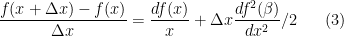
\frac{f(x + \Delta x) – f(x)}{\Delta x} = \frac{df( x )}{x} + \Delta x \frac{df^{2}(\beta )}{dx^2}/2
\end{equation}
This formula provides an error term for an approximation of the derivative when $\Delta x$ is not zero.
There are several important things to note about this formula. The first is that the Taylor series cannot be used if the function that is being approximated does not have at least two derivatives, i.e., it cannot be discontinuous.The second
is that in numerical analyis it is the power of the coefficient $\Delta x$ in the error term
that is important. In this case because the power is 1, the accuracy of the method is called first order.
Higher order accurate methods have higher order powers of $\Delta x$. In the example above only two points were used, i.e.,
$x$ and $x + \Delta x$. A three point discrete approximation to a derivative is
\begin{equation}
\frac{f( x + \Delta x) – f( x – \Delta x)}{2 \Delta x}.
\end{equation}
Expanding both terms in the numerator in Taylors series with remainder , subtracting the two series and then dividing by $2 \Delta x$ produces
\begin{equation}
\frac{f( x + \Delta x) – f( x – \Delta x)}{2 \Delta x} = \frac{df( x )}{dx} + (\Delta x)^{2} \frac{df^{3}(\beta )}{dx^{3}}/12 .
\end{equation}
Because of the power of 2 in the remainder term, this is called a second order method and assuming the derivatives in both examples are of similar size, this method will produce a more accurate approximation as the mesh size $\Delta x$ decreases. However, the second method requires that the function be even smoother, i.e., have more derivatives.
The highest order numerical methods are called spectral methods and require that all derivatives of the function exist.
Because Richardson’s equation in a model based on the hydrostatic equations causes discontinuities in the numerical solution, even though a spectral method is used, spectral accuracy is not achieved. The discontinuities require large dissipation to prevent the model from blowing up and this destroys the numerical accuracy (Browning, Hack, and Swarztrauber 1989).
Currently modelers are switching to different numerical methods (less accurate than spectral methods but more efficient on parallel computers) that numerically conserve certain quantities. Unfortunately this only hides the dissipation in the numerical method and is called implicit
dissipation (as opposed to the curent explicit dissipation).
\end{document}
[latexpage]
This is a test.
In calculus the derivative is defined as
\begin{equation}
\frac{df(x)}{dx} = \lim_{\Delta x \rightarrow 0} \frac{f(x + \Delta x) – f(x)}{\Delta x} .
\end{equation}
However, in the discrete case (as in a numerical model) when $\Delta x$ is not 0 but small, the numerator on the right hand side can be expanded in a Taylor series with remainder as
\begin{equation}
f(x + \Delta x) – f(x) = \Delta x \frac{df( x )}{dx} + (\Delta x)^{2} \frac{df^{2}(\beta )}{dx^{2}}/2
\end{equation}
where $\beta$ lies between $x$ and $x + \Delta x$. Dividing by $\Delta x$
\begin{equation}
\frac{f(x + \Delta x) – f(x)}{\Delta x} = \frac{df( x )}{x} + \Delta x \frac{df^{2}(\beta )}{dx^2}/2
\end{equation}
This formula provides an error term for an approximation of the derivative when $\Delta x$ is not zero.
There are several important things to note about this formula. The first is that the Taylor series cannot be used if the function that is being approximated does not have at least two derivatives, i.e., it cannot be discontinuous.The second
is that in numerical analyis it is the power of the coefficient $\Delta x$ in the error term
that is important. In this case because the power is 1, the accuracy of the method is called first order.
Higher order accurate methods have higher order powers of $\Delta x$. In the example above only two points were used, i.e.,
$x$ and $x + \Delta x$. A three point discrete approximation to a derivative is
\begin{equation}
\frac{f( x + \Delta x) – f( x – \Delta x)}{2 \Delta x}.
\end{equation}
Expanding both terms in the numerator in Taylors series with remainder , subtracting the two series and then dividing by $2 \Delta x$ produces
\begin{equation}
\frac{f( x + \Delta x) – f( x – \Delta x)}{2 \Delta x} = \frac{df( x )}{dx} + (\Delta x)^{2} \frac{df^{3}(\beta )}{dx^{3}}/12 .
\end{equation}
Because of the power of 2 in the remainder term, this is called a second order method and assuming the derivatives in both examples are of similar size, this method will produce a more accurate approximation as the mesh size $\Delta x$ decreases. However, the second method requires that the function be even smoother, i.e., have more derivatives.
The highest order numerical methods are called spectral methods and require that all derivatives of the function exist.
Because Richardson’s equation in a model based on the hydrostatic equations causes discontinuities in the numerical solution, even though a spectral method is used, spectral accuracy is not achieved. The discontinuities require large dissipation to prevent the model from blowing up and this destroys the numerical accuracy (Browning, Hack, and Swarztrauber 1989).
Currently modelers are switching to different numerical methods (less accurate than spectral methods but more efficient on parallel computers) that numerically conserve certain quantities. Unfortunately this only hides the dissipation in the numerical method and is called implicit
dissipation (as opposed to the curent explicit dissipation).
This is a test.
In calculus the derivative is defined as
\begin{equation}
\frac{df(x)}{dx} = \lim_{\Delta x \rightarrow 0} \frac{f(x + \Delta x) – f(x)}{\Delta x} .
\end{equation}
[latexpage]
This is a test.
In calculus the derivative is defined as
\begin{equation}
\frac{df(x)}{dx} = \lim_{\Delta x \rightarrow 0} \frac{f(x + \Delta x) – f(x)}{\Delta x} .
\end{equation}
[ tex] x = \frac{ -b \pm \sqrt{b^2 – 4ac}}{2a}[/ tex]
[tex] x = \frac{ -b \pm \sqrt{b^2 – 4ac}}{2a}[/tex]
test
[ tex] x = \frac{ -b \pm \sqrt{b^2 – 4ac}}{2a}[/ tex]
test
[tex] x = \frac{ -b \pm \sqrt{b^2 – 4ac}}{2a}[/tex]
test using latex2wp
1. A simple tutorial on numerical approximations of derivatives
In calculus the derivative is defined as
However, in the discrete case (as in a numerical model) when is not 0 but small, the numerator on the right hand side can be expanded in a Taylor series with remainder as

where lies between
  and
and  . Dividing by
This formula provides an error term for an approximation of the derivative when is not zero. There are several important things to note about this formula. The first is that the Taylor series cannot be used if the function that is being approximated does not have at least two derivatives, i.e., it cannot be discontinuous.The second is that in numerical analyis it is the power of the coefficient
  in the error term that is important. In this case because the power is 1, the accuracy of the method is called first order.
 . In the example above only two points were used, i.e.,
  and
and  . A three point discrete approximation to a derivative is
Higher order accurate methods have higher order powers of
Expanding both terms in the numerator in Taylors series with remainder , subtracting the two series and then dividing by produces

Because of the power of 2 in the remainder term, this is called a second order method and assuming the derivatives in both examples are of similar size, this method will produce a more accurate approximation as the mesh size decreases. However, the second method requires that the function be even smoother, i.e., have more derivatives.
The highest order numerical methods are called spectral methods and require that all derivatives of the function exist. Because Richardson’s equation in a model based on the hydrostatic equations causes discontinuities in the numerical solution, even though a spectral method is used, spectral accuracy is not achieved. The discontinuities require large dissipation to prevent the model from blowing up and this destroys the numerical accuracy (Browning, Hack, and Swarztrauber 1989).
Currently modelers are switching to different numerical methods (less accurate than spectral methods but more efficient on parallel computers) that numerically conserve certain quantities. Unfortunately this only hides the dissipation in the numerical method and is called implicit dissipation (as opposed to the curent explicit dissipation).
Jerry, you’ve posted on the same subject as Nick Stokes has posted on Watts UP With That, here:
It would be good if you might go there and comment. Several posters, notably angech, have suggested he is being misleading.
By the way, Jerry, you’ll probably like my paper, just published here:
https://www.frontiersin.org/articles/10.3389/feart.2019.00223/full
Pat,
I tried to post the above tutorial on WUWT but it didn’t work. Have you used larex on that site?
I also posted that Nick is not up to date on the literature. 🙂
Jerry
Hi Jerry,
I’ve never used latex, much less posted it. Perhaps you can drop a line to Charles the Moderator on WUWT, and ask about latex.
Also, Charles is the go-to guy for posting at WUWT. Essays can be sent to him, and he’ll post them up.
Pat,
read my last comment on WUWT.
Actually there may be two because one seemed to disappear.
Jerry
Pat, The post showed up briefly and then disappeared. Could Nick do that or was it Watts?
I will recreate it here if it disappears.
Jerry
Pat,
Interesting. When I asked what happened to my first post, suddenly both of them appeared. And Nick has chosen to ignore them because he has no answer for hard mathematics.
Jerry
You’ve been very busy there, Jerry. 🙂 It took awhile to find and read through all your posts.
Your discussion of the innards of the models and the dissipation problem are beyond my knowledge, though I can get a general gist of your point.
The problem of the molasses atmosphere that you raise is one that is generally ignored in all the discussions of climate models, their simulations, and their reliability.
I look forward to seeing how your conversation with Nick evolves.
In the meantime, I was happy to see that your were amused by the success of the linear emulator.
In my 2015 talk at the DDP conference, I observed that you can use a hand-calculator to duplicate the air temperature projection of an advanced climate model running on a super computerc. 🙂
Pat,
An estimate of a perturbation to the forcing of a pde yields an estimate of linear growth in time times the maximum perturbation, exactly as in youe linear model. Nick seems to have missed that fact? I can reproduce that estimate if you want.
Jerry
Will SM be commenting on these several later posts? I will be listening.
Fred,
I have written Stephen a number of messages and he has not reponded. In particular I asked him if he would allow me to post the above tutorial on a new thread, and I would like to post the estimate I mentioned above on a new thread. He has not responded, so I assumed he is busy. Thus I tried on this thread to figure out how to post the tutorial. There is a bug in CA Assistant so it took me a number of attempts. As you can see the tutorial raises a number of issues with climate and weather modelers use of numerical methods. The estimate clarifies the Stokes attacks on Pat Frank’s paper.
Jerry
It’s going to be finish of mine day, but before finish
I am reading this impressive piece of writing to improve my know-how.
I am an engineer and worked designing control systems for 37 years. Its clear to me that none of these people are adept at statistics. Their random sample studies are the stuff of basic control theory, taught in every masters degree program since the 1960’s.
“Mann and Schmidt intervened in the fray arguing in favour of ex post screening as a valid procedure.”
In the inimical words of Mandy Rice Davies: “Well they would wouldn’t they”!
7 Trackbacks
[…] Reposted from Climate Audit […]
[…] McIntyre over a Climate Audit revives a post from 2014. This site is worth a look should you be interested in some of the problems with the Climate […]
[…] https://climateaudit.org/2019/07/31/cg2-and-ex-post-picking/ […]
[…] CG2 and Ex Post Picking […]
[…] CG2 and Ex Post Picking […]
[…] https://climateaudit.org/2019/07/31/cg2-and-ex-post-picking/ […]
[…] a pedir y cuando se negaron de nuevo presentó una reclamación por mal comportamiento académico (fuente), lo que presumiblemente llevó a que Wahl y Ammann añadieran esos datos a la versión final de su […]