The following comes from Pat Frank regarding my question here
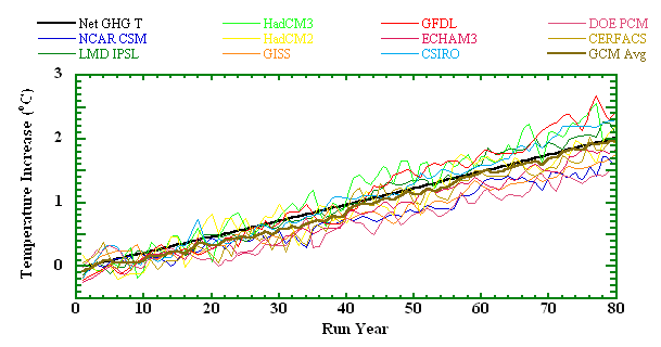
This plot shows projections from 10 of the 15 GCMs tested in the “Intercomparison of Present and Future Climates Simulated by Coupled Ocean-Atmosphere GCMs” CMDI Report No. 66. The GCM data were digitized off Figure 27 of the Report. The plot also shows the linear average of the GCM projections and the results of a simple calculation of global average temperature increase due to increases in greenhouse gases (GHGs). The acronyms at the top of the plot designate the GCMs that were used to make the respective projection, their average (GCM Avg.), and the simple calculation (Net GHG T).
The Legend to Figure 27 is: “Globally averaged difference between increasing-CO2 and control run values of annual mean surface air temperature (top) and precipitation (bottom) for the CMIP2 models. Compare with Figure 1, which gives control run values.”
And the comment on the CO2 boundary condition of the GCM projections in the text is: “To begin our discussion of model responses to 1% per year increasing atmospheric CO2, Figure 27 shows global and annual mean changes in surface air temperature and precipitation under this scenario, i.e., differences between the increasing-CO2 and control runs.” The control runs were essentially flat lines with low-intensity wiggles.
The “Net GHG T” line reflects my own calculation and assumed the same 1% per year increase in atmospheric CO2 as the GCM simulations. This calculation also included forcings from methane (CH4) and nitrous oxide (N2O). The increase in these gases was extrapolated from polynomial fits to the measured trends.
The calculation further assumed that greenhouse gasses produce 40% of the total greenhouse warming above the Top of Atmosphere temperature. This 40% includes warming due to the increased water vapor induced by the same GHGs.
The forcings for CO2, CH4, and N2O were calculated according to the equations in G. Myhre, et al., (1998) “New estimates of radiative forcing due to well-mixed greenhouse gases” Geophys. Res. Lett. 25(14), 2715-2718, Table 3.
The net temperature increase is just a linear extrapolation of the temperature from the fraction of GHG forcing in the start year (1960 in all cases), i.e., global average T is scaled by the increase in GHG forcing.
Histrorical methane was obtained from: D.M. Etheridge, L.P. Steele, R.J. Francey, and R.L. Langenfelds. 2002. Historical CH4 Records Since About 1000 A.D. From Ice Core Data. In Trends: A Compendium of Data on Global Change. Carbon Dioxide Information Analysis Center, Oak Ridge National Laboratory, U.S. Department of Energy, Oak Ridge, Tenn., U.S.A; source URL: http://cdiac.ornl.gov/trends/atm_meth/lawdome_meth.html
Historical N2O was obtained from: Khalil M.A.K.; Rasmussen R.A.; Shearer M.J.(2002) “Atmospheric nitrous oxide: patterns of global change during recent decades and centuries” Chemosphere, Volume 47(8, June), 807-821. The percent 1900 forcing was obtained by linear extrapolation of the BRW and CM data from Table 1 of the reference.
Pat’s Comment: The simple GHG-induced temperature projection goes right through the middle of the pack of GCM simulations, and closely tracks the GCM average. As the average of GCM projections is typically accounted to more accurately follow measured climate trends, the same criterion indicates that the simple GHG projection is more accurate than any of the GCM projections. It seems lots of money spent hasn’t gotten us much. One other thing of serious note: It is now obvious that GCM modelers assume that the only element driving net climate change is the level of GHG gasses in the atmosphere. This seems extraordinarily naàÆà⮶e, physically.