Lewandowsky’s most recent blog post really makes one wonder about the qualifications at the University of West Anglia Western Australia.
Lewandowsky commenced his post as follows:
The science of statistics is all about differentiating signal from noise. This exercise is far from trivial: Although there is enough computing power in today’s laptops to churn out very sophisticated analyses, it is easily overlooked that data analysis is also a cognitive activity.
Numerical skills alone are often insufficient to understand a data set—indeed, number-crunching ability that’s unaccompanied by informed judgment can often do more harm than good.
This fact frequently becomes apparent in the climate arena, where the ability to use pivot tables in Excel or to do a simple linear regressions is often over-interpreted as deep statistical competence.
I mostly agree with this part of Lewandowsky’s comment, though I would not characterize statistics as merely “differentiating signal from noise”. In respect to his comment about regarding the ability to do a linear regression as deep competence, I presume that he was thinking here of his cousin institute, the University of East Anglia (UEA), where, in a Climategate email, Phil Jones was baffled as to how to calculate a linear trend on his own – with or without Excel. At Phil Jones’ UEA, someone who could carry out a linear regression must have seemed like a deity. Perhaps the situation is similar at Lewandowsky’s UWA. However, this is obviously not the case at Climate Audit, where many readers are accomplished and professional statisticians.
Actually, I’d be inclined to take Lewandowsky’s comment even further – adding that the ability to insert data into canned factor analysis or SEM algorithms (without understanding the mathematics of the underlying programs) is often “over-interpreted as deep statistical competence” – here Lewandowsky should look in the mirror.
Lewandowsky continued:
Two related problems and misconceptions appear to be pervasive: first, blog analysts have failed to differentiate between signal and noise, and second, no one who has toyed with our data has thus far exhibited any knowledge of the crucial notion of a latent construct or latent variable.
In today’s post, I’m going to comment on Lewandowsky’s first claim, while disputing his second claim. (Principal components, a frequent topic at this blog, are a form of latent variable analysis. Factor analysis is somewhat different but related algorithm. Anyone familiar with principal components – as many CA readers are by now – can readily grasp the style of algorithm, though not necessarily sharing Lewandowsky’s apparent reification.)
In respect to “signal vs noise”, Lewandowsky continued:
We use the item in our title, viz. that NASA faked the moon landing, for illustration. Several commentators have argued that the title was misleading because if one only considers level X of climate “skepticism” and level Y of moon endorsement, then there were none or only very few data points in that cell in the Excel spreadsheet.
Perhaps.
But that is drilling into the noise and ignoring the signal.
The signal turns out to be there and it is quite unambiguous: computing a Pearson correlation across all data points between the moon-landing item and HIV denial reveals a correlation of -.25. Likewise, for lung cancer, the correlation is -.23. Both are highly significant at p < .0000…0001 (the exact value is 10 -16, which is another way of saying that the probability of those correlations arising by chance is infinitesimally small).
These paragraphs are about as wrongheaded as anything you’ll ever read.
I agree that a simple “Pearson correlation” between CYMoon and CauseHIV in Lewandowsky’s dataset is -0.25. However, Lewandowsky is COMPLETELY wrong in his suggestion that this “signal” can be separated from outliers. In the Lewandowsky dataset, there were two respondents that purported to believe in CYMoon and disagree with CauseHIV (both were in Tom Curtis’ group of two super-scammers). I’ll show that these two superscammers make major contributions to the supposed “correlation”. Like Lewandowsky, I don’t believe that these two respondents are present “by chance”: I believe that they are present as intentionally fraudulent responses.
First, the correlation can be replicated trivially as follows:
cor(lew$CYMoon, lew$CauseHIV)
#[1] -0.2547965
Second, p~+ 10^-16 can be replicated by diagnostics from an OLS regression of CYMoon against CauseHIV (standardized) as shown below:
ols=lm(CYMoon~CauseHIV,data=data.frame(scale(lew[,c("CYMoon","CauseHIV")]) ))
summary(ols)

Coefficients:
              Estimate Std. Error t value Pr(>|t|)
(Intercept)  2.574e-17  2.859e-02   9e-16        1
CauseHIV    -2.548e-01  2.860e-02  -8.908   <2e-16 ***
However, Lewandowsky is absolutely off-base in his assertion that the examination of outliers is inappropriate statistical analysis. In fact, exactly the opposite is the case: proper statistical analysis REQUIRES the examination of outliers. Furthermore, in this case, the examination of a contingency table (pivot table) is not only relevant but essential to the examination of outliers.
Examination of diagnostics by a competent statistician requires more than looking at the p-value. Part of any such analysis is examination of the qqnorm-plot for the residuals: this is the second graphic in the standard plot in R. Here are the results for CYMoon~CauseHIV (standardized), a graphic that shows severe non-normality of the residuals. (The dashed blue line shows the pattern from normal distribution of residuals.)
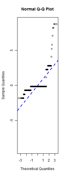
Figure 1. QQnorm- plot for CYMoon~CauseHIV.
A second basic diagnostic is examination for outliers using Cook’s distance: this is the fourth graphic in the standard plot in R. This identifies two points (889,963) as very high leverage:
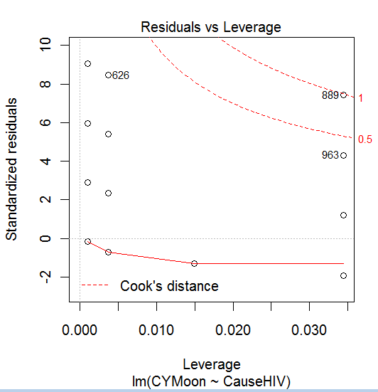
Figure 2. Cooks’ distance: CYMoon~CauseHIV.
Now, let’s do the contingency deprecated by Lewandowsky, a calculation which shows that there are only two respondents purporting to disagree on CauseHIV and to agree on CYMoon.
with(lew,table(CYMoon,CauseHIV))
      CauseHIV
CYMoon   1   2   3   4
     1   8   5 116 938
     2   1   0  33  34
     3   1   0   2   1
     4   1   0   2   3
These two respondents are the two respondents identified as outliers from the standard diagnostic (889, 963). Both are already familiar to us as super-scammers who claimed to believe in every conspiracy.
To show just that a “significant” correlation can depend as few as two outliers, I’m now going to simplify the contingency table by considering only two classes: disagree – 0 and agree-1, yielding the contingency table below: two respondents in the extreme, with 14 respondents purporting to only dispute CauseHIV and 8 respondents purporting to endorse only CYMoon, as shown below:
Data=twoclass(lew)[,c("CYMoon","CauseHIV")]
with(Data,table(CYMoon,CauseHIV))
      CauseHIV
CYMoon    0    1
     0   14 1121
     1    2    8
The (Pearson) correlation calculated in the same way as Lewandowsky is -0.1488. I’m now going to show that the two outliers dominate this calculation. (The calculation with a 4×4 matrix is structurally identical but adding up to -0.25.)
r=cor(Data$CYMoon,Data$CauseHIV); r
 # -0.1487561
There are only four unique points (0,0), (0,1), (1,0) and (1,1) in the contingency table. In the calculation below, I show the contribution of each point to the correlation coefficient. The column headed normdot is the product of (x-mean(x))*(y-mean(y)) divided by sd(x)* sd(y)* (N-1), where N is the number of respondents (1145).
N=nrow(Data)
Stat= data.frame(CYMoon=c(0,1,0,1),CauseHIV=c(0,0,1,1),count=c(  with(Data,table(CYMoon,CauseHIV)) ))
m=apply(Data,2,mean);m
Stat$dot= (Stat$CYMoon-m[1])*(Stat$CauseHIV-m[2])
Stat$normdot= (Stat$CYMoon-m[1])*(Stat$CauseHIV-m[2])/(sd(Data$CYMoon)*sd(Data$CauseHIV))/(N-1)
Stat$normsum= Stat$normdot*Stat$count
The sum of the normsum column gives the correlation coefficient.
sum(Stat$normsum)
# -0.1487561
The table calculated above therefore shows the relative contribution of each point to the correlation coefficient as shown below.
Stat[,c(1:4,6)]
  CYMoon CauseHIV count           dot      normsum
1      0        0    14  0.0086115825  0.009640767
2      1        0     2 -0.9774146183 -0.156318155
3      0        1  1121 -0.0001220419 -0.010939947
4      1        1     8  0.0138517572  0.008861259
                                       ___________
Total                                 -0.1487561
One can readily see that the two super-scammers (889, 963) contribute essentially 100% (over 100%) actually of the negative correlation between CauseHIV and CYMoon in this calculation.
Next here is the result of applying the same methodology to the 4×4 contingency table in Lewandowsky’s analysis shown here in order of decreasing contribution to the negative correlation. As above, sum(Stat$normsum) is equal to the correlation.
About half of the negative correlation comes from the 33 respondents who disagree with the Moon conspiracy and agree with CauseHIV (without strongly agreeing).
The other half of the negative correlation comes from seven outliers which contribute -0.138 (about 50% of the correlation), with the two superscammers identified above being the largest contributors. (The other 5 outliers need to be examined individually.)
There is a negative contribution from the 938 respondents who strongly agreed with HIV and strongly disagreed with CYMoon: this seems puzzling at first. What happens is that the centroid is moved off dead center. This contribution is offset relatively by positive contributions from on-axis results (CYMoon – strongly disagree or CauseHIV – strongly agree) : this seems to be fairly characteristic in this sort of sparse contingency table heavily weighted on-axis.
Stat[order(Stat$normsum),]
   CYMoon CauseHIV count    dot normdot normsum
        2        3    33 -0.761  -0.004  -0.142

        4        1     1 -8.254  -0.047  -0.047
        3        1     1 -5.425  -0.031  -0.031
        4        3     2 -2.418  -0.014  -0.027
        3        3     2 -1.590  -0.009  -0.018
        2        1     1 -2.597  -0.015  -0.015

        1        4   938 -0.014   0.000  -0.075
        2        2     0 -1.679  -0.010   0.000
        3        2     0 -3.508  -0.020   0.000
        4        2     0 -5.336  -0.030   0.000
        3        4     1  0.328   0.002   0.002
        1        2     5  0.150   0.001   0.004
        4        4     3  0.499   0.003   0.009
        1        1     8  0.232   0.001   0.011
        2        4    34  0.157   0.001   0.030
        1        3   116  0.068   0.000   0.045
Thus the “unambiguous” negative correlation between CYMoon and CauseHIV arises from the following two phenomena: about half of the -.254 comes from only seven outliers, with the two superscammers contributing the most. The other half is contributed from people who neither endorse the CYMoon conspiracy or dispute CauseHIV.
The results for CauseSmoke are very similar. The negative correlation is -0.236. A little less than half is contributed by only four outliers, especially the two (fake) outliers who purport to both strongly believe in CYMoon and disbelieve CauseSmoke. The balance is contributed from those people who hold plausible views, but did not express that they did so strongly.
   CYMoon CauseSmoke count    dot normdot normsum
        2          3    33 -0.754  -0.005  -0.149

        4          1     2 -8.231  -0.049  -0.099
        4          3     1 -2.395  -0.014  -0.014
        3          3     1 -1.575  -0.009  -0.009

        1          4   916 -0.015   0.000  -0.081
        2          1     0 -2.589  -0.015   0.000
        3          1     0 -5.410  -0.032   0.000
        2          2     0 -1.671  -0.010   0.000
        3          2     0 -3.492  -0.021   0.000
        4          2     0 -5.313  -0.032   0.000
        1          2     5  0.149   0.001   0.004
        1          1     4  0.232   0.001   0.006
        3          4     3  0.343   0.002   0.006
        4          4     3  0.522   0.003   0.009
        2          4    35  0.164   0.001   0.034
        1          3   142  0.067   0.000   0.057
Far from the examination of contingency tables being irrelevant to the analysis, they are essential to it.
The “signal” from Lewandowsky’s analysis is also “unambiguous”: that, using his own words, “number-crunching ability that’s unaccompanied by informed judgment can often do more harm than good”. A thesis that his own work amply illustrates.
Update: Jeff Id asked about the effect of robust regression. I’m working on a longer post on robust regression, but will preview this with the result here. R has a very handy robust regression function rlm in the same style as lm, the default option is Huber’s robust regression. The “robust” correlation between CYMoon and CauseHIV is the robust regression coefficient between standardized versions of each series: the robust correlation is 0.000000 (not Lewandowsky’s -0.254). Lewandowsky’s “unambiguous” result is unambiguous dreck.
fm=rlm(CYMoon~CauseHIV,data=data.frame(scale(lew[,c("CYMoon","CauseHIV")]) ))
summary(fm)
            Value         Std. Error    t value
(Intercept) -2.433000e-01  0.000000e+00 -2.138241e+09
CauseHIV     0.000000e+00  0.000000e+00 -2.938290e+05

Residual standard error: 5.487e-09 on 1143 degrees of freedom