I’ve had a longstanding interest in high-resolution ocean proxies (with posts as early as 2005 – see Ocean Sediment tag) and had already written detailed reviews of many of the individual high-resolution series used in Ocean2K (e.g. here here here here here here). In these prior discussions, the divergence between the 20th century proxy data and 20th century instrumental data had been a major issue. The non-bladedness of Ocean2K data was therefore unsurprising to me.
Although, for their main figures, the Ocean2K authors made the questionable decisions to voluntarily degrade their data both into 200-year bins and from deg C to SD units, in their Supplementary Information, they identified a network of 21 series with high-resolution extending into the 20th century, showing results in 25-year bins but only for the short period 1850-2000, once again re-scaling, this time using only six values (25-year bins) for each series.
In my first post, I had undertaken to examine their data in higher resolution and will do so today using their high-resolution network – without the needless re-scaling and over the entire 0-2000 interval. The results clearly confirm the absence of a 20th century blade. The Ocean2K authors were singularly uninformative about this obvious result; I’ll show how they worked around this “problem”. I’ll also discuss untrue claims by Ken Rice (ATTP) and other ClimateBallers that the Ocean2K data “finishes in 1900” or is otherwise too low resolution to permit identification of a concealed blade.
Background: the Ocean Proxy “Divergence Problem”
I had initially become interested in high-resolution ocean data (especially alkenone and Mg/Ca, rather than dO18) because, as opposed to tree rings, they were directly calibrated in deg C according to standard equations (not ex post correlations).
Alkenone series are based on the ratio of C37:2 and C37:3 in coccolithopores, while Mg/Ca series are based on ratios in foraminifera, with surface dwelling foraminifera (especially G. ruber) being of interest. During the past 20 years and especially the past 10 years, alkenone samples have been widely collected throughout world oceans and coretop and sediment trap calibrations yield sensible maps of ocean temperature without jiggling. In deep time, they also yield “sensible” results. Alkenone series constitute 15 of 21 high-resolution of the Ocean2K dataset (26 of 57 overall) and also the majority of the Marcott ocean data (31 of 60), with foraminifera Mg/Ca being the second-largest fraction.
Alkenone and Mg/Ca series had originally been collected to shed light on “deep time”, but there were occasional box cores which both preserved the most recent sediments (a sampling problem with piston cores) and which had been sampled at sufficiently high-resolution to shed light on the past two millennia. I’ve made a practice of regularly examining the NOAA and Pangaea datasets for potentially relevant new data and, over the past 10 years, had already noticed and separately discussed many of the series in the high-resolution Ocean2K dataset (e.g. here here here here here here).
Here, for example, is a figure from Leduc et al 2010, previously shown at CA here, showing dramatic decreases in alkenone SST at two sites: Morocco, Benguela. (Both these sites are included in the Ocean2K high-resolution dataset, both with more than thirty 20th century values.) Numerous other CA posts on the topic are in the following tags: Ocean sediment; Alkenone.

Figure 1. From Leduc et al 2010. Both locations are in the Ocean2K high-resolution network.
In a number of CA posts, I had questioned the “alkenone divergence problem”, the term alluding to the notorious divergence between instrumental temperatures and tree ring density proxies that had given rise to various “tricks” to “hide the decline” in Mann’s section of IPCC TAR and other articles in order not to “dilute the message”. In important ways, the alkenone divergence problem is even more troubling as (1) there is a physical calibration of alkenone proxies, whereas tree ring densities are merely correlated after the fact; and (2) alkenone proxies have “sensible” properties in deep time.
The “problem” arising from divergence between a proxy reconstruction and instrumental temperature is that such divergence makes it impossible to have confidence in the proxy reconstructions in earlier periods without reconciling the divergence. Mann, for example, has always insisted that his reconstructions have statistical “skill” in calibration and verification periods, though the validity of such claims has obviously been at issue.
A Reconstruction from the Ocean2K “High-Resolution” Dataset
The Ocean2K data consisted of 57 series of wildly differing resolution: nine series had fewer than 20 values, while twelve series had more than 100 values. In geophysics, specialists always use high-resolution data where available and use low-resolution data only where better data is unavailable. In contrast, in their main figures, the Ocean2K authors degraded all their data into 200-year bins and made composites of the data only after blurring.
In their Supplementary Information, the Ocean2K authors identified a subset of 21 high-resolution series: twelve of the 21 series had more than 20 values in the 20th century, seven series had more than forty 20th century values and all but one had more than eight values. In Figure S10, they showed a high-resolution composite in 25-year bins, but only for the 1850-2000 period and only in SD Units (1850-2000 and only after binning).
Because the underlying proxy data is already in deg C, it is trivially easy (easier in fact) to do the Ocean2K calculations in deg C rather than SD Units and it’s hard to believe that the Ocean2K authors hadn’t already done so. Figure 2 below shows the composite of high-resolution ocean cores in 25-year bins over the 0-2000 period (rather than 1850-2000) and in deg C (rather than SD units.) For comparison, I’ve also shown instrumental HadSST (black) and the composite from the full network in Ocean2K technique using 200-year bins (but retaining deg C). Expressed in deg C, there is a major divergence in the 20th century between instrumental temperature and the proxy reconstruction. Even late 20th century proxy values are clearly below medieval values.
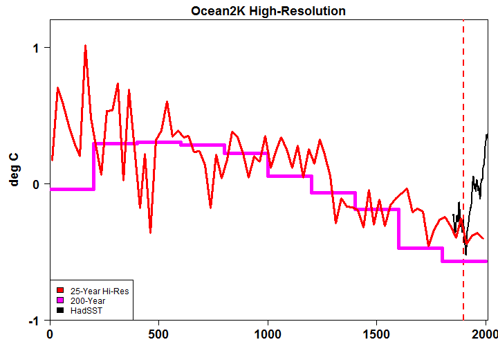
Figure 2. Red – 25-year bin composite of Ocean2K high-resolution ocean cores (not using one incongruous singleton coral series) retaining deg C. Magenta- composite for full network, calculated as in Ocean2K composite, but retaining deg C throughout. Black – HadSST global (since ERSST global series only begins in 1880.)
McGregor et al made no mention of this dramatic divergence in their main text, instead asserting that “the composite of reconstructions from tropical regions are in qualitative agreement with historical SST warming at the same locations”:
Although assessment of significance is limited by the number and resolution of the reconstructions, and by the small amount of overlap with historical SST estimates, we find that the composite of reconstructions from tropical regions are in qualitative agreement with historical SST warming at the same locations (Supplementary Fig. S10). Upwelling processes recorded at a number of the sites may also influence the twentieth-century composite (Supplementary Sections 1 and 8).
Even if the tropical composite was in “qualitative” agreement (a point that I will examine in a future article), this implies that the extratropical divergence has to be that much worse in order to yield the actual overall divergence. It is very misleading for the authors to claim “qualitative agreement” in the tropics without disclosing the overall divergence.
Deep in their Supplementary Information (page 44), they quietly conceded that the high-resolution composite did not yield the warming trend of the instrumental data, but there is no hint of this important result in the text of the article:
The 21_O2k and 21_Kaplan composites are non-significantly correlated (r2 = 0.17, df = 4, p = 0.42), with the warming trend in the 21_Kaplan not reproduced in the 21_O2k composite (Supplementary Fig. S10).
They illustrated this with the following graphic (in 1850-2000 SD units after binning). While the use of SD Units degrades the data, even this figure ought to have been sufficient to dispel the speculation of some ClimateBallers that the 1800-2000 bin might combine low 19th century values and high 20th century values, thereby concealing a blade.

Figure 3. Excerpt from Ocean 2K SI Figure S10, showing Kaplan SST (top panel) and Ocean2K high-resolution composite, both expressed in 1850-2000 SD Units (after binning).
While the SD units of the 200-year bin and 25-year bin figures are not the same, I think that it is still instructive to show the two panels with consistent centering. In the figure below, I’ve centered the panel showing the 25-year bins so that it matches the reference level of the final (1800-2000) bin of the 200-year reconstruction, further illustrating that its final bin does not contain a concealed blade.

Figure 4. Left panel – Ocean2K in 200-year bins (PAGES2K FAQ version from here); right – bottom panel of SI Figure S10a, with its zero value aligned to value of 1800-2000 bin in left panel. Both panels in SD Units (not deg C). I’ve been able to closely emulate results in the left panel, but not as closely in the right panel.
The Supplementary Information carries out corresponding analyses on subsets of the high-resolution data: tropical vs extratropical, upwelling vs non-upwelling, alkenone vs Mg/Ca. Trying to analyse the divergence through such stratification is entirely justified, though the actual statistical analysis carried out by the Ocean2K authors is far from professional standard. I’ll discuss these analyses in a separate post. For now, I’ll note that similar concerns have been raised about alkenone data in a Holocene context, even by Ocean2K authors. Lorenz et al 2006 (discussed at CA in early 2007 here) had contrasted trends in tropical vs extratropical alkenone data over the Holocene; in my commentary, I had pointed out the prevalence of upwelling locations in the tropical data.
Postscript: False ClimateBaller Claims that the Data “Finishes in 1900”
In reaction to my first post, Ken Rice (ATTP) and other ClimateBallers argued that there was no reason to expect the Ocean2K data to have a blade, since the data supposedly ended in 1900 or was otherwise too low resolution. Such claims were made at David Appell’s here, at Rice’s blog here and on Twitter.
As I observed in my post, the Ocean2K data archive is excellent and the measurement counts easily calculated. A barplot of measurements (grey) and cores (red) is shown below. Not only does the data not end in 1900, the number of individual measurements from the 20th century is larger than any previous century. Nor is this sample too small to permit analysis. 21 series are considerably more than the number of medieval proxies in many canonical multiproxy studies that are uncontested by IPCC or ClimateBallers. While it would be nice to have more data (especially in the Southern Ocean), there’s easily enough 20th century data to be worthwhile discussing.

Figure 5. Number of measurements in the Ocean2K dataset by 20-year period (grey); number of contributing series by 20-year period (red).
Now consider various assertions about the data made by Rice and others. Shortly after my original article, Rice stated (here and here) that the data ended in 1900 and thus there was no reason to expect a blade.
“As far as I’m aware, it finsishes in 1900 and the paper has “pre-industrial” in the title. So why would we expect it to have a blade?”
Rice even accused me of “misread[ing]” the x-axis:
Can’t quite work out how you’ve managed to misread the x-axis so badly?
I informed Rice in a comment at Appell’s that his belief that ended “in 1900” was incorrect as follows:
Ken says: “As far as I’m aware, it finsishes in 1900 and the paper has “pre-industrial” in the title. So why would we expect it to have a blade?” The data doesn’t end in 1900. There are more measurements in the 20th century than in any previous century. The 20th century data doesn’t have a Hockey Stick either, as you can see in their Figure S10a.
I had also posted a Twitter comment highlighting that, even in the Ocean 2K step graph, the final (1800-2000) bin of the step-graph extended to 2000. Rather than defend his false claims, Rice made a Gavinesque exit, but not before making an unsupported allegation that I was spreading “misinformation” about the Ocean2K study:

Nonetheless, a few days later, Rice returned to the topic in a blog article on Sept 13, re-iterating his untrue claim that the Ocean2K data ended “in 1900”:
Steve McIntyre (who was involved in the discussion on David Appell’s blog) seems to be highlighting that the recent Ocean2K reconstruction does not have a blade. Well, the data appears to end in 1900 and the paper title is Robust global ocean cooling trend for the pre-industrial Common Era, so why would we expect there to be a blade.
This time, one of his readers (improbably, Sou) pointed out to Rice that the 1800-2000 bin must include 20th century data. Sou speculated that 200-year bin could contain a concealed blade in the bin through a combination of cold 19th century values and warm late 20th century values – apparently unaware that this possibility had already been foreclosed by Supplementary Figure S10):
I don’t know that the recent ocean2k paper ended in 1900. I think what it did was end in the 1801 to 2000 “bin”, which would have included the coldest years of the past 2,000 years, as well as whatever proxy records were included up to 2000. The boxes in Figure 2 showed a lot of things, including the median for each 200 year bin, the latest of which was centred on 1900 – but went from 1801 to 2000.
Rice amended his post to say that his prior assertion (that the data ended in 1900) wasn’t “strictly correct”:
What I say here isn’t strictly correct.
However, the issue is not that his original assertion wasn’t “strictly correct”; the issue was that it was unambiguously wrong.


150 Comments
Text reading
Rice stated (here and here)
has no link at the second “here”.
Observer
As long as we’re checking links — the 3rd in your series of 6 CA links is malformed, and (if the syntax is fixed) duplicates the first. [In both locations, paragraphs 1 & 6.]
Steve, excellent article. Another case study in the manipulation of data to obtain “correct” but nonetheless dubious results. Thus the Ocean2K data shows clearly that there was no 2K SST warming, no ocean hockey stick.No wonder Leduc got rattled: he could see it coming.
###
Is this a typo?
A Reconstruction from the Ocean2K “High-Resolution” Dataset
The Ocean2K data consisted of 27 [57?] series of wildly differing resolution
Steve: thanks. fixed.
Ocean2K news release:
Actual paper: Proxy data in the paper shows nil 20th century warming and the (“20 times faster”) instrumental data the quote is based on has nothing to do with the study. If one can ignore resolution, for instance, then one can interpret a high tide as a super-accelerated sea level rise.
Mentioned only deep in supplementary information: they quietly concede that the high-resolution composite did not yield the warming trend of the instrumental data…
Steve, is there any explanation of the authors or others as to why the divergence problem in the 20th century? It actually looks like they start to track well from 1880-1910.
The only flaw I see in your work, Steve, is a typo: “1900 or was otherwise to low resolution.” Too, not to. Otherwise perfection. (STeve : fixed.)
Steve: In order to explain the divergence problem, they would first have to clearly report it. They did analyse tropical vs non-tropical, upwelling v non-upwelling and alkenone v Mg/Ca, and these analyses were undoubtedly inspired by the divergence problem, but were weakly done. For example, one thing to look at is whether divergence was localized to upwelling zones and didn’t impact the rest of the ocean and whether proxies were heavily biased towards upwelling zones. That doesn’t seem to be the explanation, but it’s the sort of thing that one has to look at. Right now, I’m unaware of any convincing explanation. I, for one, am reluctant to too quickly reject otherwise interesting proxies and would have appreciated a thorough examination of the issue by Ocean2K authors.
Steve — Very interesting, if unexpected results! I have three questions —
First, how can it be that for the last 400 years, the 200-year averages of the 25 year bins do not come close to the corresponding 200 year bin values in your Figure 2 above?
Second, how did you compute anomalies of the individual series? The method they describe on p. 24 of the SI incorrectly flattens any reconstruction, since they set the mean of the binned values for each series over its own period to zero. Instead, one should only do this for the longest series that span the entire 2000 years. Then, each shorter series should have its mean set equal to the mean, over its own short period, of all longer series. I pointed this out in the earlier discussion at
And third, what happens if a series only has values in two non-adjacent bins? Does it make no contribution to the intermediate bin, or is its value there filled in by interpolation?
Hu, I always enjoy your comments.
You say:
As far as I know, the 25-year bins only involve 21 series selected from the whole.
w.
Steve: yes. Also the Ocean2K 25-year bin high-resolution composite appears to have been calculated without an intermediate step of calculating of individual ocean series. I did the same. So the two series are related, but not identical. I had originally done this figure as a two-panel diagram with one panel showing the SD and SST 200-year bins and carrying one forward to the panel shown here, but decided that it was too confusing.
Willis —
Thanks. That would do it, and would also answer my third question, since I suppose series with gaps of more than 25 years have been excluded from the 21. Also, the paucity of such series in the distant past would account for the great volatility of the high-frequency reconstruction back there.
I’m still concerned about the spurious flattening caused by zeroing each short series relative to its own period, however.
Steve: I’ve done a check in which the center for each series was treated as a random effect, also calculating a random effect for each period as a cross effect. This seems to me to be a more rational way of doing the calculation, but I didn’t want to move too many parts at once. I’ll try to post on this. It tends to smooth things, but does not change the medieval-modern relationship.
I replicated their methods as closely as possible to minimize the number of moving part. I don’t endorse their techniques but the larger issues seem insensitive. Their composite appears to be a weighted average of six ocean composites, each of which is a simple average of scaled series, scaled after binning. They do not appear to have interpolated between non-adjacent bins, but this is an obvious permutation that is more of an issue when lower resolution series become involved.
In their 25-year bin composite, it appears to me that they directly constructed the composite without intervening ocean averages.
In the top panel of the figure below, I show my near-exact emulation of their SD unit 200-year reconstruction, also showing the 200-year bin SST reconstruction (magenta) without rescaling. (Scale in right axis). Only nuances of difference in the general shape. In the lower panel, I show the figure shown in the above article, carrying forward the (magenta) 200-year bin reconstruction in deg C units.
I think Craig Loehle neatly handled the problem of unequal frequency data in our 2008 paper (he did the reconstruction and I just added the se’s): He interpolated every series to an annual frequency, averaged them, and then took tridecadal averages. He accepted series that had as few as 20 observations in 2000 years, but even observations 100 years apart shed information on the big picture of climatic change. Most of them had far more observations, justifying a finer resolution in the average.
In retrospect, however, I now think that it would have been better if he had just reported bin means as in McGregor et al, rather than moving tridecadal averages, in order to make it very clear that there was no annual precision to the reconstruction. It would also have made it clearer that our final point of 1935 in fact represented data from 1920 or so to 1950.
See http://www.econ.ohio-state.edu/jhm/AGW/Loehle/ .
Steve, Many thanks for this very interesting article. I look forward to your intended future posts analysing subsets of the high resolution data.
One question. Whilst I don’t doubt that Alkenone and Mg/Ca proxy temperature data is much more reliable than tree ring data, do you have an idea of how good it is, especially in terms of the magnitude of any drift over time in the relationship with local ocean temperature?
Steve: I’ve seen contour maps of the world ocean constructed from core top alkenones and the results were impressive. I’ll try and locate one. Also, alkenone series (and Mg/Ca) series over the Pleistocene have impressive correlations with Vostok ice core results. The coherence of such disparate proxies gives me considerable re-assurance that they are actual PROXIES rather than squiggles.
Nic, Conte et al “Global temperature calibration of the alkenone unsaturation index (UK′37) in surface waters and comparison with surface sediments” http://onlinelibrary.wiley.com/doi/10.1029/2005GC001054/full shows calibration of alkenones. Here is plot of coretops from all over the world ocean – very different calibration than tree rings.
SteveN, the Conte paper would appear on my fast perusal to support my supposition that the alkenone, like O18 for ice cores, proxies can differentiate large changes in temperatures – as used in their study- but that we would expect large variations using much smaller ranges of changes as those ranges appear for millennial changes. I have assumed here that the periods of comparison between ice cores and alkenone proxies were over interglacial periods.
The paper also points to the process of sedimentation as a source of variability that is probably less well understood than the chemical saturation effect. Also excluding 3 standard deviation outliers without explantion is troubling.
Steve: I didnt try to provide a reading list. This article was not the basis of my comment about deeo time. Look at Iberian Margin cores for an example.
Rice actually thought the data ended in 1900 despite all of your hints otherwise and then the actual paper itself? Wow. Andthentheresidiots.
And sure, the focus of the paper wasn’t to show a 20th century blade…but if the methodology and/or data were truly apples-to-apples with 20th century warming, then obviously it should appear.
I can see Sou’s point where a cool 1800-1900 period combined with a 1900-2000ish blade would be somewhat concealed through the use of a 200 year binning process, but as you note, the information was there to disprove that.
Do these people now know how to read?
The thing is that they need it to be spoon fed to them (as do I) but they cant accept it because it goes against their beliefs. They cant see big red markers in papers like “200 year binning” which people like Steve immediately see as a concealing and obfuscating mechanism whereas AGW enthusiasts see as nothing more than a choice.
Thanks Steve. These divergences are disastrous for paleoclimatologists. And most of them dont even know it (publicly)
Steve: I’m not nearly as prepared as many readers to declare a pox. The alkenone data has some impressive results geographically and in deep time. I regard the 20th century divergence as a problem and a puzzle. On the other hand, the Ocean2K results unequivocally refute the Marcott blade from similar data, though the O2K authors carefully walked by this nettle.
So, one scientist remains.
…and Then There’s Integrity
Well I take “problem and puzzle” to its scientific conclusion and regard the 20th century divergence as a problem that invalidates the proxies as reliable temperature measures until such time as the causes can be found and reliably countered.
Until that time, IMO, proxies are of interest only. And I’m especially disappointed by claims that, for example, the MWP was more or less warm than present or that the current warming is at an unprecedented rate.
Steve: don’t get me wrong on this. I regard unresolved divergence problems as fatal to efforts to use proxy comparisons to assert that the modern period is warmer than (say) the medieval period or Holocene Optimum. It’s not the only issue: bristlecones don’t have a divergence problem, but that doesn’t mean that they are uniquely valid proxies for world temperature. Note that I do not assert that Lamb’s squiggle is revealed truth either.
Shouldn’t bristlecones be considered as diverging in the other direction?
Of course, the ocean2k data is not needed to refute Marcott’s spike – Marcott’s own data and his Phd thesis suffice.
Sure, but the “O2K authors carefully walked by this nettle” and they shouldn’t have.
Very interesting is your fig.1, showing the “divergence” of the alkenone data derived from two upwelling zones off west Africa. These upwellings involve a type of current known as an Eastern Boundary Current: the Canary Current, a southward flowing current offshore of Morocco and the Benguela Current, a northward flowing current offshore of Angola.
If one accepts the reliability of the data (there is no reason not to), then it can be concluded that the rate of upwelling has increased this past century at these two core locations. Eastern boundary currents are wind-driven and the upwelling is due to a force known as the Eckmann Effect (or Eckmann drift or pump), a phenomenon associated with such currents. These Eastern Boundary Currents are variable and fickle, so it cannot be precluded that the sampled locales would show a twentieth century cooling as a result of long-term trend in these currents, with consequent implications for climate. All very interesting.
To explain, the rate of upwelling can be expressed in meters/day and, typically, may be 5 to 10 meters/day. Thus the rate of upwelling determines the time spent in the photic zone and this determines the amount of insolation/warming the upwelling water undergoes in its migration from the cold depth to the surface. An increase in the rate of upwelling should lead to cooler SST, as this lessens the duration of exposure to insolation/warming of the upwelled water.
It has occurred to me that I should expand this comment and state my premise: that is,the “divergence problem” of an alkenone series derived from areas of upwelling could be explained by long-term trends in upwelling rates. Thus the alkenone proxy would be correctly recording actual changes in SST, and the so-called “divergence” problem becomes no problem.
Of course, this hypothesis needs support and as Steve commented above:
“one thing to look at is whether divergence was localized to upwelling zones and didn’t impact the rest of the ocean and whether proxies were heavily biased towards upwelling zones”
Lots of work remains to be done regarding verification of alkenone data reliability as a SST proxy. I see much promise in the technique.
This might be an error. Steve wrote: “In a number of CA posts, I had questioned the “alkenone divergence problem”, the term alluding to the notorious divergence between instrumental temperatures and tree ring density proxies ” …
The part after “the term alluding to” phrase seems to describe the tree ring divergence problem.
In defense of Mr. Rice, he said, As far as I’m aware, it finishes in 1900
I think this could be a reasonable belief looking at the data depicted in the 2000 year graph. The data indeed does not exceed the 19th century.
Mr. Rice says again, responsively, Well, the data appears to end in 1900
Well, again, the data does appear to end at about 1900. In the 2000 year graph. Is it unreasonable to scientifically accept this depiction as full disclosure of the data available? I think this could be a reasonable belief. I do not think Mr. McIntyre’s previous blog post citation to Mr. Rice, as you can see in their Figure S10a [b?] is enough notice to Mr. Rice. Not many have time to read the Supplemental Report, let alone a busy presentation of six binning boxplots effectively buried at page 46. Besides, why should someone’s cite to the supplementary material be assumed to negate an assertion or implication in the overlying report? Should not, in science, the supplementary materials be assumed to support the report?
After a poster named Sou mentions the last 200-year bin stretches to 2000 a.d., Mr. Rice says,
What I say here isn’t strictly correct.
I think this is an contextually reasonable statement of perplexity. Some posters here in the previous CA thread also struggled to find a valid reason why there was an 1800-2000 year bin, but no data depicted therein past 1900, assuming there was no deception in the representation. Accordingly and additionally, “binning” is an esoteric statistical art–I believe–unfamiliar to many–I have seen, including me–a situation which complexifies clear comprehension. Which, of course, may have been an underling intention.
Steve concludes, the issue was that it was unambiguously wrong.
If the issue is whether 20th century data was available, the answer is yes, such is wrong. I viewed it in Excel, and it was immediately apparent there was plenty of 20th c. data. If the issue is whether 20th century data was depicted, besides at page 46 in the supplementary material, that question is “ambiguous.” No proxy data was depicted after 1900 within the last bin, but said bin extended to 2000.
Mr. Rice, and others, are victims of the underlying game of hiding-the-no-cline. I suggest they accept my approach as the empirically-grounded reasonable scientific standard suited for climate science: Assume B. S. Assume any graphic depiction omits, misstates, or makes up something important. If things go visibly missing, like data lines after 1900, assume a bad purpose. Always check the hard data, and always assume the supplementary materials are the place to hide negative information. Always assume negative information is possibly but obscurely disclosed, as such obfuscating tactic provides, at least to the propagators’ minds, plausible deniability.
Two more points about Supp Figure S10:
1. The 6 so-called 25 year bins look to be half-that years length wide. Is this a product of aesthetics, or is the actual data used therein not 150 years worth, but only about half that.
2. Was the Kaplan SST (obscure TMK) used because its blade is minimal compared to others, say HadSST? That is, did the supp information desire not to show too much divergence?
FollowTM says:
“Mr. Rice, and others, are victims of the underlying game of hiding-the-no-cline. I suggest they accept my approach as the empirically-grounded reasonable scientific standard suited for climate science: Assume B. S. Assume any graphic depiction omits, misstates, or makes up something important. If things go visibly missing, like data lines after 1900, assume a bad purpose. Always check the hard data, and always assume the supplementary materials are the place to hide negative information. Always assume negative information is possibly but obscurely disclosed, as such obfuscating tactic provides, at least to the propagators’ minds, plausible deniability.”
###
Excellent advice, the credo of a skeptic, but good luck on getting “Mr. Rice and others” to pay any heed. My impression is that Mr. Rice will never be part of the solution and, indeed, he is not a victim, unless one sees him as self-victimized.
“…In defense of Mr. Rice, he said, As far as I’m aware, it finishes in 1900
I think this could be a reasonable belief looking at the data depicted in the 2000 year graph. The data indeed does not exceed the 19th century…”
Really? I thought it was quite clear from Steve’s post on Sept 4 that there was data beyond 1900. Steve made it pretty clear this was true to Mr. Rice, and Mr. Rice kept insisting it wasn’t, going so far as to tell Steve, “Can’t quite work out how you’ve managed to misread the x-axis so badly?”
“The data indeed does not exceed the 19th century.”
Yes, it does. It calculates (what it claims is) an average from 1800-2000, and labels this average “1900”. How is this hard? I mean, you might not know it from looking at the graph but you would know if you did a little reading.
“Mr. Rice says again, responsively, Well, the data appears to end in 1900”
Correct, if you are just looking at a graph without reading. Which is not a time to shoot your mouth off arrogantly about how somebody else ‘badly misread’ that which you didn’t read at all.
“What I say here isn’t strictly correct.”
What he says here is wholly and entirely and unambiguously false, and it came from shooting his mouth off without reading.
Until he admits that he had no clue what he was talking about, a fairly sizable INR (Imperial Nudity Rating) should be considered to apply to anything he says. He has been shown to shoot his mouth off and then not admit his mistake, covering it up by loudly asserting that anyone who notices the nudity of the emperor must be a ‘denier’.
I suppose I am doing the same since the paper is paywalled and I am just going by what others say here. If it can be shown that the others are wrong I’ll take this back.
“the paper is paywalled…”
Available here thanks to Dr. Leduc.
Supplementary information here.
Thanks! Look forward to reading it. However, I only had to glance at the first page to see:
“…each SST reconstruction was averaged into 200-yr
‘bins’ (that is, 200-yr averages for 1–200 ce and so on, up to
1801–2000 ce; “.
So.. yeah.
Rice being unambiguously wrong is not unusual. It’s his trademark.
It is indeed a mystery though about the divergence. Would seem a worthy topic for careful analysis. Steve, you seem to not really speculate about this. Any thoughts?
Rice: “What I say here isn’t strictly correct”.
Translation: “What I say here is wrong”. Add: “As is normal for me”.
Rice is obviously very intelligence.
What I say here isn’t strictly correct, of course…
Regarding the divergence, It seems to me that it would not be so dramatic if the surface temperature record adjustments had not enhanced the anomaly.
The question that has to answered to my way of thinking then is which is the more reliable indicator of actual global temperature anomaly (if there is such an entity). The temperature record or the ocean proxies.
Terry,
Temperature record or ocean proxies the best?
Since one has been calibrated against the other at some stage of evolution of the method, the argument is in danger of circularity.
Thanks, SteveM, for the thought provoking post. I would agree that there are non-tree ring temperature proxies that have much more straight forward interpretations than tree rings. Even so it appears that divergences can be found in these non-dendro reconstructions. Even Mann (2008) admitted to divergence not only in dendro but non-dendro proxies as well. The admission was a rather off hand comment in the paper that was buried in the text and with no effort to explain.
I would suspect the reason we do not see attempts to explain divergences in proxies in the papers involving temperature reconstructions is that its mention has to draw attention to the looming issue that divergence without explanation logically kills any conclusions from the temperature reconstruction about modern versus pre-modern warming. An explanation that might retain historical validity would require that the divergence be readily related to AGW effects like increasing CO2 levels in the atmosphere or other anthropogenic effects uniquely realized during the period of divergence. I have seen weak handwaved explanations, but all were conjectures and far from convincing.
All of the above leads me to ask a few questions:
What are the chances that a paper dealing with dendro or non-dendro divergences could be readily published?
At what point and with what evidence would a divergence problem be merely considered evidence that the proxy and temperature relationship does not hold sufficiently for a temperature reconstruction?
Are some of these non-dendro proxy divergences with better behavior when correlated with O18 from ice cores a matter of magnitude of temperature change and temporal resolution?
How about conjecturing on potential divergence causing processes and the validity of those processes?
Ken, You hit the nail on the head. Paleoclimatology is trying to ignore or conceal the divergence problem. Thus one side of the AGW debate ignores divergence, accepting the pre-instrumental proxy hockey stick handle attached to the instrumental blade. Without a hypothesis for the 20th century proxy withering, (across multiple proxy mechanisms,) there is no avenue to start such an investigation. And, without an explanation for the proxy 20th century proxy divergence from instrumental one must either invalidate the proxies or invalidate the instrumental. Steve points out here: “…alkenone series (and Mg/Ca) series over the Pleistocene have impressive correlations with Vostok ice core results. The coherence of such disparate proxies gives me considerable re-assurance that they are actual PROXIES rather than squiggles.”
If the proxies are valid the logic leads to one to the otherwise dark theory of massively biased instrumental adjustments. I would not be surprised if there were bias but we know from historical accounts that rivers that froze in the 17th and 18th century every winter do not always freeze today, while the figure above Steve provided shows the proxies reporting about the same global temperature. Of course, the LIA could have been a regional event (northern hemisphere) as CAGW proponents readily claim.
Did anyone else notice that the volatility of the first 500 years as compared to the last 500? Could this be a clue? Could there be a trend of flattening proxy sensitivity? And, whether or not that is so, I notice a lot of 20X 100-yr slopes relative to the 2000-yr slope. Evan knew this and intentionally misled the public. Where does bias end and misconduct begin?
Ron Graf —
“Did anyone else notice that the volatility of the first 500 years as compared to the last 500? Could this be a clue? Could there be a trend of flattening proxy sensitivity? ”
As I noted above at https://climateaudit.org/2015/09/19/the-blade-of-ocean2k/#comment-763425 , this big decline in the volatility of the average of the 21 high-resolution proxies in Steve’s Figure 2 above is probably just due to the much smaller number of high-resolution proxies in the first 500 years relative to the last 500 years. His Figure 5 above shows that the density of observations has been much higher since about 1200 AD, and especially since 1700 AD. Averaging a smaller number of proxies makes the average have a higher variance. Furthermore, the impact of a proxy leaving the average (going backwards in time) is much bigger when there are only a small number of remaining proxies. (Steve’s Figure 5 is drawn for 20-year bins rather than 25-year bins as used in Figure 2, but the implications are similar.)
If all 57 proxies were included by interpolation as Craig did in Loehle and McCulloch (2008), these effects would be very much reduced, as the earlier period would have many more proxies. See https://climateaudit.org/2015/09/19/the-blade-of-ocean2k/#comment-763430 .
In any event, the great reduction in volatility of the aggregate is just do to the increasing availability of data of the type used for the figure, rather than any flattening of proxy sensitivity.
Thanks Hu. I see at the 1250 AD mark where data density doubles is the last major swing. This takes Evans off the hook for ignoring the plot as evidence of actual temperature swings yet it can’t excuse assuming their absence.
The divergence problems of the proxy climate studies seems to be widespread. Is this the case in other areas of science, and how is it dealt with if it is?
Some other divergence problems in science. Men report more sexual partners than women, but this is impossible. Someone is lying. People report themselves more willing to spend money on schools than when they vote on a bond issue for schools. Early radiocarbon dates gave odd results for older samples until they found the source of some of the problems. The observed expansion of the universe conflicts with other aspects of the physics and motions of galaxies conflict with their estimated mass–they are vigorously searching for a solution and don’t pretend it is not there.
If you find your instrument (survey, lab equipment) is out of calibration or giving odd readings, you try to fix it before using it further.
In science, divergence is a discussion point, not a problem…
What ever happened to the pleasure of finding stuff out?…
Because “Climate Science” is settled…
You can come up with a “novel” method that mines proxies for hockey sticks, and that helps. It’s not wholly adequate, though, so you creatively hide-the-decline by obscuring or eliminating periods of divergence.
As a layman, the impression from the comments and the article is that the Alkenone proxies, etc are showing less warming that the air/surface.temperatures, ie a divergence problem for the late 20th century. This raises a few questions:
1) how do the proxies compare to the ocean temps as measured by the argo system and/or to the prior ocean temp measuring system (pre Argo’s)
2) The world temps have been on a steady decline since circa 1300 AD through circa 1850 AD which most proxies tend to confirm (tree ring, ice cores, alkenone, etc). The O2k study likewise confirms the general cooling during this period. With respect to the divergence problem, Any thoughts that amo/pdo may have a slight counter effect to the ocean temps as compared to the surface temps? (though not enough to hide/mask the long term warming or colling trend, but enough to mask the short term cooling and/or warming trend?
The Calvo et al (alkenone based) study off the coast of southern Australia seems to show similar results to Antarctic temp during the Holocene.
This study seems to show a reduction in SST over the last 7,000 years and is in agreement with other studies from this area.
There are a number of graphs here that seem to show this SST decline. Any comments?
Click to access 12.pdf
Here’s a question I’d like answered. How much instrumental global warming has there been since 1850? To me the HAD 4 data seems to show about 0.8 C. But is this data accurate or not?
Alkenones are produced by phytoplankton such as Emiliania huxleyi. These simple plants convert CO2 into alkenones. The thermal calibration is based on the temperature of the mixed layer. The mixed layer is in contact with the atmosphere. At any given atmospheric level of CO2, the dissolved concentration of CO2 increases as temperature falls, so the phytoplankton live in a “richer” CO2 environment when the temperature is lower. If the alkenone unsaturation ratio is due to the differences in availability of dissolved CO2 at different temperatures, the the “divergence” of alkenones could just be due to rising atmospheric CO2, with the higher dissolved CO2 masquerading as lower temperature. It is interesting too that there are differences in upwelling regions… those Are regions where the dissolved CO2 is not in equilibrium with the atmosphere, and is in part influenced by the CO2 concentration in the deeper ocean.
A controlled experiment in the laboratory with growth of Emiliania huxleyi at different CO2 partial pressures and different temperatures, along with measured alkenone unsaturation might explain the divergence since 1900.
So Steve is the HAD temp data accurate since 1850 or not. And how can you test that accuracy over the last 165 years?
My comment is about a possible cause for the divergence this post discusses, not about the accuracy of the historical SST record (Hadley or other). That said, the gradual rise in sea level over the 20th century is at least consistent with warming and thermal expansion, though clearly some of the sea level rise is from melting of land supported glaciers and pumping of groundwater. I don’t think anyone knows the exact contribution of each.
Steve, Aussie blogger Ken Stewart has looked at a number of regions of the planet and using UAH V 6 satellite data has calculated the length of the pause for each.
The planet has not warmed for 18 yrs 5 mths.
The NH has not warmed for 18 yrs 2 mths.
The SH has not warmed for 19 yrs 7 mths.
The Tropics have not warmed for 21 yrs I mth.
The Tropical oceans have not warmed for 22 yrs 11 months.
The North polar region has not warmed for 13 yrs 7 mths.
The South polar region has not warmed for 36 yrs 9 mths or for the entire record.
Australia has not warmed for 17 years 11 mths.
The USA has not warmed for 18 yrs 3 mths.
So where is the impact from extra co2 emissions? And why hasn’t the South polar region warmed at all since 1979?
RSS has been diverging from HADCRUT4 since 2005, joining UAH. Plot here.Has anyone heard an explanation? If not, how far can it diverge without needing one?
Not sure what point you are trying to make. Do you think that there has been no warming of the ocean surface since the 1800’s? If so, on what basis do you draw that conclusion?
Neville,
I agree with SFP, your response to his experiment design suggestion seems to be non sequitor. Did you respond to the right comment?
I’m amused that Bill Clinton once called CO2 ‘plant food’, but only once. I think he couldn’t resist the dig at Al Gore.
So, Steve F, we’re not even seeing man’s warming effect in the ocean at all if your surmise is correct. That’s discouraging.
==========
kim,
If the cause for the divergence could be identified and quantified, then perhaps it could be taken into account in the alkenone record. It’s always better to understand what is happening than not understand.
For what it’s worth, this strikes me as a plausible explanation for at least part of the divergence. It also seems like the kind of thing that might be testable in the lab. Has anybody looked?
While they’re at it, they may wish to cast their eyes over the isomerization chemistry of alkenes and ketones by UV.
Steve, you say:
“If the alkenone unsaturation ratio is due to the differences in availability of dissolved CO2 at different temperatures, the the “divergence” of alkenones could just be due to rising atmospheric CO2, with the higher dissolved CO2 masquerading as lower temperature”
###
That seems very unlikely.
The “divergence” examples Steve provided above come from upwelling water: water which is “pristine” and unaffected by present day atmospheric CO2 levels.
The occurrence of alkenone “divergence” in upwelling water must have some other explanation.
Well risen water, to the light, and CO2 diffuses rapidly.
==========
A well-referenced article by Schouten at al gives some of the many factors thought in year 2000 to influence the relation between temperature and alkenone properties.
Click to access Mix_etal_2000_g3_alkenones.pdf
It is accepted that the art will have progressed in the 15 years since. I hope so, because the uncertainties listed by Schouten do not place the use of alkenones on a secure footing as a temperature proxy. There are numerous other variables that need to be quantified if the method is to give temperature estimates. In year 2000, the link between T and alkenone properties would not seem to be capable of giving better that +/- 1 deg C of resolution, about the same as hypothesised global temperature change in the lat 100 years.
As I noted in a previous post, the Conte paper linked by SteveM shows a graphic of temperature versus alkenone proxy response that appears very applicable for tracking large changes in temperatures like would be expected from glacial to inter glacial periods, but when you are looking for 1 degree C changes, as would be expected over a 2000 year past period, the variation of proxy response to temperature from the Conte paper would appear to make that not practical or valid unless a large number of replicate samples were used. Given the Conte data that would be an interesting analysis.
I suspect that if the stevefitzpatrick conjecture of anthropogenic increasing CO2 levels could be shown to cause divergence as he has suggested that any number of climate science authors would be publishing results. After all it would be just this kind of divergence cause that would keep the historic part of the temperature reconstruction intact – with everything else being equal. After perusal of the Conte paper I would have my doubts on the use of alkenones for accurately tracking the relatively small temperature changes expected in the last 2000 years even if a reasonable explanation for the divergence could be found. Alkenones and O18 fractions appear capable of tracking the expected temperatures of the interglacial and glacial periods, but both have divergences in some reconstructions from the instrumental period. The divergence could be and perhaps would be more readily considered as merely a random response of a proxy rather insensitive to relatively small temperature changes if we did not have the expectation and evidence that the recent response should be to a rather large temperature change. The same goes for tree rings where divergence could be merely a sign of a proxy response incapable of tracking temperature above an apparent random level.
I have not yet read the link from Geoff Sherrington on alkenone response to temperature
So far, the only alkenone “divergence” that I have seen is in the samples taken from areas of upwelling, posted by Steve above. If the “divergence” is found only in such samples (from upwelling), then these samples might be recording actual SST and hence the “divergence” problem is nil. See my comment above.
Geoff —
It would indeed be foolhardy to use a single such series to measure global or even local temperature swings (as in “David Appell’s cherrypick” discussed in Steve’s previous post). However, the average of 25 such series will have only 1/5 the variance of a single such series, etc (if we may assume the variances are finite), so that there is hope that a suitable composite of several proxies will be meaningful.
Hu McCulloch, you might want to look at the graphs in the Conte paper link from a SteveM post above. The graphs to which I refer are for the alkenone to temperature relationship before and after sedimentation. The before relationship shows a best case range of approximately 10 data points (with near the same alkenone response) in the middle region of temperature of 2 to 3 degrees C and at the low and high end temperatures a range with the approximately the same number of data points as the middle of an eyeball of around 6 degrees C. After adding in the variable of sedimentation the ranges in the mid temperatures nearly double and the proxy to temperature relationship varies much more with region.
The Helen V. McGregor paper does not even reference the Conte paper.
Looking closer at the references of the McGregor paper I see that there are none that have presented data related to variability of the proxy response to temperature variability of the proxies used in their reconstruction. This is not unusual unfortunately with papers dealing with temperature reconstructions. The authors seem to rush to some conclusions about climate without much bother to look in detail at the proxies they use.
It will be interesting when I have time to use data from sources giving variability of proxy response to temperature over a range of temperatures – like in Conte – and doing a Monte Carlo simulation to determine the statistical significance of the trend in the McGregor paper.
Mr. McIntyre: I have a naive question. In Fig.4, left panel, the SD is the greatest in the most recent 200-year bin, the bin which also contains the most counts (right panel) of any bin. This seems crazy to me. Unless I am totally not understanding it, this aspect of Fig. 4 seems to be saying that the more measurements taken, the “worse” the result. Can you explain this?
William —
“In Fig.4, left panel, the SD is the greatest in the most recent 200-year bin, the bin which also contains the most counts (right panel) of any bin. This seems crazy to me. Unless I am totally not understanding it, this aspect of Fig. 4 seems to be saying that the more measurements taken, the “worse” the result.”
This might just be an artifact of the way the series were standardized by McGregor, Evans, Leduc et al. A short sample from a highly persistent series will typically have a lower variance about its own mean than a longer sample will. Swings in the shorter sample will therefore spuriously get greater weight in the composite of standardized series than will comparable swings in the longer samples. Since the shorter series are concentrated at the recent end of the period, there is more overall variability there in the standardized scores. Note also that the boxes in Figure 4a represent the quartiles of the data before averaging, not the standard error of the mean.
I doubt that a similar graph using the raw temperatures rather than sd units would show this effect.
Mr. McCulloch:
Thank you for responding to my question–much appreciated. This is certainly fascinating stuff.
Steve, is bioturbation addressed anywhere with these high-resolution cores? Calculated temperatures are presented as point estimates at exact dates, however activities of marine benthos even in high-sedimentation regions will mix the top several centimeters of sediment continuously, spread the foraminifera vertically, combine older and younger specimens at each level, and make age-dating more uncertain. Binning, at least with small ranges, won’t help matters because of overlap at the edges of the bins.
Good point on bioturbation. I have seen ocean cores (photos, that is) and these tend to be laminated and show any bioturbation quite well. But some cores show very little bioturbation or none. My point is that there is “high resolution” and otherwise categories for these alkenone series and presumably the investigators are familiar with such problems. I could be wrong, however.
Stuck in moderation, second try.
#####
I would suppose that those in the ocean core business take full account of any disturbance in the sediments which could alter results. Such core studies have been ongoing for over half a century.
“It’s not the only issue: bristlecones don’t have a divergence problem”
I don’t think that is exactly right, Steve. Bristlecones don’t have an apparent divergence problem vis-à-vis temperature, but that might be due to aliasing by the CO2 fertilization effect.
stevefitzpatrick, from the link above provided by Geoff Sherrington, we have the following comment: The carbon isotopic composition of alkenones or other organic compounds combined with those of foraminifera offer the potential to reconstruct the distribution of aqueous CO2 concentrations in the upper ocean (Figure 4)
It appears that an estimate of what would be required for the testing of your conjecture on CO2 changes might be available to climate scientists. Later in this comment from above the authors point for the need to know the temperature also and suggest using alkenones. This might get circular for historic times, but might be useful if ocean CO2 concentration variations are sufficiently wide in the instrumental period and measured. The article lists secondary effects on the alkenone response to temperature and does not mention CO2 concentration differences.
Yes, I saw that too. what they did not do was look at any effects of CO2 concentration on the unsaturation ratio used to estimate temperature…. they considered C12/C13 ratio only. I found other papers which suggest (based on lab growth) that pH above 8.8 severely inhibits growth (starved for CO2!) but at any pH below about 8.3 growth is limited by other factors (like nutrients). I can find no references which explore the effect of available CO2 on unsaturation
Steve, since the authors suggest determining pCO2 using carbon isotope ratios and factoring that by using the alkenone unsaturation ratio for a temperature proxy and all from the same organism, they must assume that pCO2 and alkenone unsaturation are independent.
Kenneth,
I agree that they seem to assume that. I just haven’t seen anything in the quick search I did to say that is in fact correct. There are a number of factors which have been identified which influence unsaturation ratio, so maybe someone evaluated partial pressure of CO2….. I just haven’t seen a reference.
Ken,
The possible response to CO2 raises a problem for most proxies.
We calibrate from temperature that is most reliable over the last 50 years or more.
Yet, this period is described as anomalous for CO2 concentrations.
It is hard to calibrate when two parameters, T and CO2, are not behaving in a way considered normal for a thousand years or more beforehand.
Posted Sep 23, 2015 at 4:38 AM | Permalink
Not clear what you mean by this. While CO2 is well outside its historical range, and thus could be an issue for alkenone calculations, I’ve never seen a scrap of evidence showing that temperatures “are not behaving in a way considered normal for a thousand years” … do you have a citation for that claim?
All the best to you,
w.
Hi Willis,
I am referring to the widespread belief in global warming. I do not accept it verbatim. If one does, then it could be said that both T and CO2 are anomalous and not showing the patterns of previous centuries.
I think I am right in saying that if a calibration produces (say) a linear response with a slope of 2 when it should be one, then the proxies calibrated from it will be 0.5 of the correct value. And vice versa. In reference to the “hiatus”, if the slope is zero, then one can do no calibration over the period of the hiatus. For this reason, proxy results should not be used for the last 15 years or so, with the possible exception of when the Temp pattern locally shows little hiatus.
One can do SOME calibration. A ‘proxy’ that jumps all over the place while temperatures stay about the same ain’t that great a proxy.
somebody get me a sweater.
McGregor et al made no mention of this dramatic divergence in their main text, instead asserting that “the composite of reconstructions from tropical regions are in qualitative agreement with historical SST warming at the same locations”:…Even if the tropical composite was in “qualitative” agreement (a point that I will examine in a future article), this implies that the extratropical divergence has to be that much worse in order to yield the actual overall divergence. It is very misleading for the authors to claim “qualitative agreement” in the tropics without disclosing the overall divergence.
The paper has a thin oily film of facial plausible deniability here. It cites “Supplementary Fig. S10.” Actually, it is Supp fig. S10g “Tropical composite” that is on topic. But by omitting g I was compelled to look at all of S10’s graphs and found h “Extra-tropical NH composite” which shows industrial era decline. Sooo..they disclosed the divergence to all readers responsible enough to assume material information is being hidden or obscured.
Explication of the tropical/extra-tropical divergence here would be fascinating scientifically. But the authors seem to prefer to play hide the ball for the sake of the lucrative anthropogenic greenhouse gas game.
I looked at the Blogpost above and saw this little gem planted by a ‘dumbscientist’ dated 20th Sept.
“I’m no dendrochronologist, but Wikipedia’s overview seems helpful. Mann, Park & Bradley 1995 didn’t scale proxy records to obtain temperature, but MBH98 was the first to use a scale factor determined by principal component analysis of the proxy records vs. instrumental record PC’s during the calibration period from 1902 to 1980.
It would be even more interesting to know if it’s ethical to quietly change the scale (and units) of the MBH98 reconstruction graph to hide it among a cherry-picked 1% of simulations based on input noise with much longer decorrelation time than the US Congress was told.”
It could be obvious who this is by admitting he is ‘no dendrochronologist’
Dumbscientist’s comments have a peculiar shrill tone to them reminiscent of one W……. who is found stamping his trademark tone all over blogdom.
Unlike some, including yourself, I always post under my own name and sign all of my comments. Whoever “dumbscientist” might be, he/she has nothing to do with me. As to you throwing mud, that’s a sure sign you’re out of real ammunition …
w.
When will Willard wonder well?
========
Willis I was not thinking of you see kim
Huh? Who is Willard? And since Kim’s comment is the first mention of “Willard” in the thread, it’s still unclear what you were referring to ..
w.
To get up to speed, see links in Steve Mc’s postscript. Willard is shrill. Dumbscientist, too. Peas in a pod.
Thanks for the further information, mpainter. I try to never go to “And Then There’s Peabrains”, it makes my head hurt.
In any case, this is why I always ask people to quote what they are referring to … mistaken identity and unclear references are the bane of online discussions, leading to endless misunderstanding.
So … I appreciate you clearing up that misunderstanding.
w.
De nada.
Reblogged this on I Didn't Ask To Be a Blog.
An article about the use of particle accelerators to probe isotopes in minute quantities had this to say about foraminifera analyses:
http://arstechnica.com/science/2015/09/the-particle-accelerator-that-can-draw-data-out-of-specks-of-comet-dust/
Pat Michael’s “World Climate Report” shows here how much warmer the Holocene climate optimum was than temps today.
The MacDonald et al study found that forests grew up to the Arctic coastline during that period and temps were several degrees C higher than our present warming.
http://www.worldclimatereport.com/index.php/2006/05/25/more-evidence-of-arctic-warmth-a-long-time-ago/
Neville, just to bring the contrary view, the argument is the LIA and MWP were NH events. Does anyone have references to tree ring studies in the Andes or other SH evidence? And, the Holocene optimum is explained by orbital cycles (Milankovitch). So the consensus argument is orbital influence is cooling Earth now with sporadic pauses (chaotic variability), but not supporting a century-and-a-half-long 0.8C climb.
BTW, I would have thought Ocean2K would have attributed the 2K decline to M-cycle, but they don’t. Instead they put it on “models validated” volcanic aerosols. I guess for the authors the data signal is clear as a bell. Or, maybe they shunned risk of paying gratitude to CO2 for averting a 100K-year glaciation.
If the claim is that orbital influence is cooling Earth with sporadic pauses, doesn’t it follow that the only reason there wasn’t an “MWP” is because before it, things were even warmer?
Does anyone have references to tree ring studies in the Andes or other SH evidence?
Click to access CookPalmer.pdf
Thank you Matt. I’d seen that before but misplaced the link.
Matt,
Australia lacks publications in which new proxy information is reported. The reason evades my. I am cynical enough to suggest that proxy work that has been done does not tell the ‘right’ story and so is not published. Even in the full 2K, very little if any is on the Australian mainland, with a little of Ed Cook’s dendro work on Huon pines in Tasmania, where the problems of finding a reasonable temperature record are off-putting.
And to be counter contrary, while it often asserted the MWP and the LIA were regional events limited to Western Europe and the Northern Atlantic, it appears places like Alaska, the Yukon, Chile, South Africa, Siberia and New Zealand must have moved since then to where they are today.
Ron the Calvo study found a warmer Med WP in S OZ and the PAGES 2K study also found that Antarctica was warmer than today from 141 AD to 1250 AD.
1250 AD is surely a good fit for a SH Med WP. Also there are a number of S America and NZ studies that show a warmer Med WP as well.
Steve
Is it unnecessary to analyze the high resolution dataset regionally vs globally?
Regards
Richard
In a comment on the last article here, at https://climateaudit.org/2015/09/04/the-ocean2k-hockey-stick/#comment-763058 , I pointed out that McGregor, Evans, Leduc et al misuse the Wilcoxon signed rank test for the median difference between pairs of observations, thereby greatly overstating the significance of bin-to-bin temperature changes.
I have now looked at the textbook they cite, in order to check whether it leaves some ambiguity as to how to perform the test, or even mis-represents it. The source they cite is Statistics and Data Analysis in Geology, by John C. Davis, 2002.
Although the Davis text discusses the related Mann-Whitney-Wilcoxon rank sum test for the equality of two distributions, it in fact makes no mention at all of the signed rank test itself. They must therefore have based their test on a different source.
Two standard treatments of the signed rank test, Wilcoxon’s own article in Biometrics Bulletin, 1945, and the influential textbook by Siegel and Castellan, Nonparametric Statistics for the Behavioral Sciences, 2nd ed, 1988, make it quite clear that with n matched pairs, the test looks only at the n differences of pairs, not at the n^2 differences drawing from matched and unmatched pairs. McGregor et al. actually go one step further, by even including several observations that are not part of matched pairs.
While I am confident that there was significant climate change before the modern CO2 period, and would be surprised if this data did not support that conclusion, arriving at a correct conclusion by using bad statistics is bad science, even if it is “peer reviewed” and published in Nature Geoscience.
Hu –
Is it possible that the authors used the MWW test and merely mis-stated the name of the test? From your earlier comment, it seems that they computed the Hodges-Lehmann statistic for the two time bins; that is, the median of all pairwise differences.
Harold —
Thanks for the reference. What they in fact computed was indeed the Hodges-Lehmann (or H-L-Sen) statistic for the difference of two populations, which I had not heard of before your post. However, the H-L statistic takes no account of the fact that the paired differences have much smaller variance than the unpaired differences. The Wilcoxon signed-difference test takes this into account by using only on the relatively very small number of paired differences.
The Kirchner reference you give provides a large sample normal approximation to test whether the difference is zero, that takes into account the high variance of the differences, under the assumption that the matched pair differences have the same high variance as the unmatched pairs. However, what McGregor et al said they did was to compute z-scores using the Wilcoxon signed difference normal approximation, but using the much larger sample size of the Hodges-Lehmann statistic. This enabled them to get off-the-chart significance from data that in fact had only marginally significant evidence of climate change.
Whatever statistic McGregor (mis)used it does not take into account the variability of the proxy response to temperature and further, at least for alkenones, that variability becomes very large towards both ends of the temperature range. I would have carried out a Monte Carlo simulation to determine confidence intervals using the published proxy/temperature variability for the expected site temperature – and even if available data on response variability limited the simulation to alkenone proxies which make up nearly half the 57 reconstruction sites. Of course, I am looking at the results from skeptical point of view while with the McGregor authors probably not so much.
Also the Magnesium to Calcium ratio proxies in McGregor which with alkenones make up almost all the proxy data have a high resonse variability to temperature as shown in the linked paper here:
http://www.whoi.edu/cms/files/hbenway/2006/6/Barker
QRS(2005)_11406.pdf
I had a chance yesterday to look at this. I ran the turnkey Matlab program provided by McGregor et al. It ran without problems, reproducing figure 2a of the paper, and producing the 200-year-binned averages. However, the script did not cover the calculation of bin-to-bin changes of Section 7 of the SI.
I first tried to replicate the McGregor et al. calculation. I computed {d_ij} = { ( x_i – y_j )/2 } where {x_i} is the set of standardized values in the later bin, and {y_j} in the earlier bin, and applied the Wilcoxon signed-rank test (Matlab function “signrank”) on the {d_ij}. [Divide by 2 to compute change per century, as the bins are separated by 200 years.] I obtained slightly different results than those of section 7. Section 7 results are in parentheses below.
Bins dT z(dT) p(z_dT)
100- 300 -0.03 (-0.03) -2.19 (-2.51) 0.03 (0.01)
300- 500 -0.07 (-0.07) -2.94 (-3.58) 0.003 (0.0003)
500- 700 -0.02 (-0.01) -1.65 (-1.79) 0.10 (0.07)
700- 900 -0.04 (-0.04) -1.60 (-1.56) 0.11 (0.11)
900-1100 -0.07 (-0.07) -5.85 (-5.34) <1E-5 (<1E-5)
1100-1300 -0.17 (-0.17) -15.29 (-14.80) <1E-5 (<1E-5)
1300-1500 -0.17 (-0.18) -14.83 (-14.54) <1E-5 (<1E-5)
1500-1700 -0.06 (-0.06) -4.14 (-3.84) 0.00003 (0.0001)
1700-1900 +0.07 (+0.08) -5.87 (5.61) <1E-5 (<1E-5)
That's reasonably close, although it's surprising to see any differences using their data and a simple two-step procedure.
I attempted two alternative tests. First, I used the signed-rank test on matched pairs, for proxies with data in both bins. ["signrank" with two arguments.] The result:
Bins Number z p
100- 300 29 -0.18 0.86
300- 500 33 -0.26 0.80
500- 700 38 -0.34 0.73
700- 900 43 -0.22 0.83
900-1100 44 -0.58 0.56
1100-1300 45 -3.14 0.002
1300-1500 43 -2.34 0.02
1500-1700 40 -0.52 0.60
1700-1900 39 -1.39 0.16
Much more believable z-values, and only two changes are significant at p<0.05.
The second alternative was to apply the Wilcoxon rank sum method (equivalent to the Mann-Whitney "U" test) to the binned sets, using the Matlab function “ranksum”. This gave the following result:
Bins z p
100- 300 0.33 0.74
300- 500 0.62 0.54
500- 700 0.15 0.88
700- 900 0.48 0.63
900-1100 -0.89 0.37
1100-1300 2.29 0.022
1300-1500 -2.41 0.016
1500-1700 -0.63 0.53
1700-1900 0.53 0.59
Again, only two significant changes at p<0.05.
This is rather deeper statistical waters than I am used to wading in, so I leave discussion of the best methods to others. Offhand, though, it strikes me as a stretch to consider the set of standardized scores in a bin as deriving from a single distribution, as the proxies have been standardized over different periods. [Exhibit A: the two-bin proxies which are coerced to values +/-0.707.] This makes any test somewhat suspect, in my naive opinion. Perhaps if the proxy series were standardized before binning?
I agree with you that the method of McGregor et al. overstates the number of degrees of freedom in the set of {d_ij} and hence the significance.
One more. Using the Hodges-Lehmann-Sen statistic per the Kirchner reference above, the median and 95% range for the bin-to-bin change is (in std.dev./century)
100-300 -0.03 (-0.31 to +0.19)
300-500 -0.07 (-0.29 to +0.16)
500-700 -0.02 (-0.20 to +0.17)
700-900 -0.04 (-0.19 to +0.11)
900-1100 -0.07 (-0.23 to +0.09)
1100-1300 -0.17 (-0.32 to -0.02)
1300-1500 -0.17 (-0.31 to -0.04)
1500-1700 -0.06 (-0.23 to +0.11)
1700-1900 +0.06 (-0.18 to +0.38)
In only two cases, the 95% range excludes 0.
Harold —
Excellent! I wonder, however, if there aren’t a couple of sign typos.
In your first table, you give the z-stat for 1700-1900 as -5.87, whereas McGregor et al got +5.61. Is one of you wrong on sign? Shouldn’t the z-stat have the same sign as the HLS point estimate?
In your second table, you give the z-value for 1700-1900 as -1.39, even though Figure 2a and the HLS estimate (with corrected p-values in your fourth table in your second post) show a weak increase during this period. Should this be positive?
And finally, the signs in your third table seem all mixed up — 1100-1300 and 1300-1500 look like they both showed declines in Figure 2a, yet your table has the former strongly positive and the latter strongly negative. However, I think this may be a quirk of the way that the rank-sum statistic is sometimes computed. Siegel and Castellan in their influential textbook compute their statistic as the rank sum of the smaller of the two samples, just for convenience in tabulating the exact distribution. From 1100-1300 the sample grows from 45 to 49, so that an above average statistic would mean that 1100 is higher on average than 1300. However, from 1300 to 1500 the sample falls from 49 back to 44, so that an above average statistic would instead mean that 1500 is higher on average than 1300, while a below average statistic, as apparently obtained, would mean that 1300 is generally above 1500. The online documentation for Matlab ranksum seems to indicate that if the exact distribution is used, the test statistic represents the first series given to it, whichever is larger. But then under the large sample approximation, it states that “n_x” is defined to be smaller than “n_y”, so I’m not sure which they’re doing.
Hu –
Good eyes on the signs! I noticed the oddities when transcribing the Matlab output into the comment. I double-checked at that time, but edited out a note about them, as the comment was already quite long. I just now re-checked: the z-values are as Matlab produced them.
Regarding the first two tables, this article at Stackoverflow mentions that the z values from “signrank” are not sensitive to the sign of input arguments, which is unexpected but unimportant if you’re interested in p-values. The z-value signs in McGregor Table S13 (SI Section 7) are more sensible — perhaps McGregor et al. used Octave, and Octave handles the signs in a more logical manner than Matlab. I have a machine at home with Octave; I’ll try to run the same script tonight to see if there’s a difference.
For the third table (ranksum), this article mentions that for Matlab versions 2012a and older — which includes the version I was using — the z-score is inverted if the 2nd vector is shorter than the 1st vector. Again, counter-intuitive.
P.S. Apologies for the table formatting. It was nicely lined up before I hit submit, but apparently multiple spaces are changed to single spaces.
Other than a motivation to obscure why would anyone bin 200 years of data in a paper that is obviously aimed at understanding historical climate with reference to the modern and instrumental warming period. We have had essentially a short period from the 1970s to 2000 or so of rapid warming that would of course get lost in taking 200 year bin represenations of temperatures.
A quick look at the plots of temperatures in McGregor would tend to support the papers that list the variability of alkenone and Mg/Ca ratio proxy responses to temperature. It would assume the variability is a normal distribution and the division of the standard deviation by the square root of n to obtain the standard error reported in McGregor is derived using n as the number of different proxy sites. I am not at all certain these assumption apply.
If I wanted to determine the trend (linear or otherwise) over the past 2000 years using the McGregor data why would I not merely plot all data using the expected given the temporal resolution?
Hu –
I tried the same process in Octave.
First, I ran the turnkey script of McGregor et al. It threw a divide-by-zero exception, but seemed to produce the 200-year-binned reconstruction all right.
It took a little effort to translate the Matlab tests for bin-to-bin changes to Octave, as neither “signrank” nor “ranksum” exist in Octave, but there are equivalents in “wilcoxon_test” and “u_test”. The signs of the z-values are more sensible, being negative for all changes except 1700-to-1900, for all test versions. I noticed slight numerical differences, e.g. z=+1.39 vs. z=-1.37 for the matched-pair Wilcoxon signed-rank test for the 1700-to-1900 change. Still couldn’t reproduce McGregor et al.’s Table S13 precisely; e.g. the last change gave z=5.87 vs. z=5.61 of Table S13.
Of course, all of this is inconsequential to the larger goals of the paper.
Hu, Thanks. Your research seems to have very important implications for the paper’s statistical claims and credibility in general. When you answered my earlier question about the declining volatility in the high-res proxies being explained by lower sampling in the earlier intervals, is that sudden drop in volatility (in response to more data density) an effect that would be typically present if the p values were as claimed by the authors? If not, wouldn’t this have been easily apparent to anyone with a statistical background?
Ron —
The sudden drop in volatility you refer to is in Steve’s Figure 2 above, which is not in the original paper. The authors therefore made no claim about it, one way or the other.
On the ATTP discussion at David Appell’s blog, I saw the repeated mention of the meme that the red-noise hockey sticks produced by M&M (or Wegman) were a cherry-pick of one out of a hundred results from the actual random algorithm. I thought that was an interesting claim at the time, and don’t recall that there was a rebuttal. (And you see that it is still being actively repeated.) Was there a rebuttal?
The claim is Climateball invention. And, yes, Steve did address and refuted the claim on that Appell thread. See link above in Postscript.
Since I don’t really understand the claim, it would be good to see something more like: here is exactly what you are claiming, you are missing the following, and only then – here is figure such-and-such in MM that proves it.
Since this is a frequent claim by that group, I think it would be helpful to have a place where the response is made fully.
“Not strictly correct” falls well within the margin of error for “unambiguously wrong”.
😉
I wonder what the modelers are going to do now with their preindustrieal runs.
The news release claims the instrumental record (blade) is alarming evidence of AGW by comparing its 20X slope to the smoothed 2K reconstruction, when it fact the study shows, with its higher resolution data portion, 20th century-like slopes could have been commonplace. Yet, ironically, the study’s own 20th century proxies show a limp blade, diverging without explanation from the instrumental record, opening new (unaddressed) questions about the validity of either the proxies or the instrumental record.
As Steve opines, the presentation of the reconstruction would have been plenty large enough endeavor to warrant publication. Yet the authors chose to delay and add to the team, compelled to present it with an explanation for the downward 2K trend. From the news release their model analysis proved: “Only volcanic events resulted in a cooling trend that matched the team’s real-world observations.” But within the paper the authors rightly point out that heat is the integral of ALL forcings, not just volcanic. Their model analysis also includes orbital, land use (deforestation), solar and greenhouse gas, the later diminishing (I assume due to uptake by colder, less saturated oceans).
My question:
1) Why the need to dismiss all but volcanic effects?
2) Where is the source for the assumption that Earth has been experiencing anomalously high volcanism over the last 2K years?
3) How does one assume orbital influence can turn on and off?
4) Aren’t ocean currents conspicuously missing from the list?
I have finally had some time to look at the individual proxy series in McGregor (2015). In analyzing the individual proxy series in temperature reconstructions I have found that the detail there can often more efficiently reveal problems with the proxy response to temperature than the more generalized discussion that is most often seen in the main body of a temperature reconstruction publication.
What I have noted in the individual proxy series of McGregor is that if one plots a long term regression trend straight line (with some over periods of hundreds of years) over the entire time period of the proxy data (without binning) is that I visualize residuals around that line that appear to be randomly distributed with in some cases the distribution appearing additionally in a cyclical and/or strong auto correlation pattern. Maybe I am seeing something in a biased manner and thus I want to show these graphs of the time series of the individual proxies with the straight regression trend lines in a couple of posts here with the hope that there remains some belated interested readers who might give me some feedback. The graphs are to be posted along with tables that show the detailed results of the analyses and cross referenced to the graphs.
The first of two groups of individual proxies selected consists of 16 proxies that that have response data into the modern warming period. Like the other individual proxies in McGregor some of these trend slopes are pointed downward, some upward and some with zero significant trends and with most being downward pointing (and thus providing the conclusion in McGregor). What is most interesting is that except in maybe 2 or 3 cases the trend line with the scatter of points around it shows little or no deviation in the modern warming period. Visual deviation for 2 of those exceptional cases could be due to the higher frequency of data in the modern warming period.
My problem with these long term trends of greatly varying slopes over long periods of time and trends seemingly unaffected with the known instrumental data upward trends in the modern warm period is that all these observations could be interpreted as the proxy response or measurement of the proxy response responding to something other than temperature. It is difficult for me to accept that on a long term basis of hundreds of years that we would see this large a variation in temperature trends at specific global locations. Further why do these trends want to continue in the same direction into the modern warming period where we have instrumental data strongly showing that this should not be the case.
The key to this analysis should be analyzing the regression residuals with the details of auto correlation and distribution the auto regression residuals. Unfortunately the irregular time series in McGregor have to be converted to regular series before carrying out these analyses and I have not had time to do this yet. I plan to use the zoo function in R to do this with the caveat that the final analysis can depend heavily on how I do the zoo conversion. The scatter of the residuals around the trend line shown in these series is not unexpected given the know response variation to temperature of these proxy types and the fact that the sedimentation and sampling of it must be doing some averaging of individual years.
In this post I will show the 16 modern warming proxy data analyses with a table and 4 graphs. In the next post I will show the similar analysis results from the 24 individual proxies that effectively have data in the year 1000 to year 1900 range.
Links to table and graphs for 16 modern warming era proxies:
Table Of Results:

Graph1 of 4 Proxy Series with Trendline:

Graph2 of 4 Proxy Series with Trendline:

Graph3 of 4 Proxy Series with Trendline:

Graph4 of 4 Proxy Series with Trendline:

Second post of 24 individual McGregor proxy series from 1000 to1900 with table and graphs linked below:
Table Of Results:

Graph1 of 4 Proxy Series with Trendline:

Graph2 of 4 Proxy Series with Trendline:

Graph3 of 4 Proxy Series with Trendline:

Graph4 of 4 Proxy Series with Trendline:

Graph5 of 4 Proxy Series with Trendline:

Graph6 of 4 Proxy Series with Trendline:

I have a couple of posts in moderation and with SteveM’s apparent absence from the blog I will make these posts without the linked graphs – which I surmise is what put the posts into moderation. The reason I am doing this is because I need some feedback on the proper handling of irregularly spaced time series as appears in the proxy data used in McGregor (2015). I have done some simulations with time series that I judge are close emulations of the McGregor series to determine whether I can get reasonably close results for determining trends with a regularly spaced series and then simulating the spacing that I see in some worst case McGregor proxies. I have assumed that irregular spaced data results in McGregor are the results of an averaging effect from the sedimentation and thus my simulation from regularly to irregularly spaced series uses an average of the missing data spaces. I have found that for the simulations of some McGregor series that the slopes of a straight line regression are very nearly the same for the simulated regular and irregular series. The p.values for the slopes are somewhat higher for the regular than the irregular series which I take to mean that the extra degrees of freedom obtain in the regular series outweighs the averaging effect in the irregular series.
In a preceding post I was hoping to convert an irregular series (the residuals from the regression of the series) to a regular one using the zoo library and function in R. I see that is not really possible for what I want to do. I ask anyone here for a proper method of conversion and whether conversion would be advisable in this case. I think Hu McCulloch referred to preferred ways of handling these problems. Also is my assumption that the irregular increments in the McGregor series can be handled as averages. Finally the graphs of some McGregor proxy series with the trend line indicates to me that the proxies show reasonably consistent long term trends of widely varying values that to me indicates some long term effect on the proxy response or measurement that is not related to temperature. I would like to hear comments on the appearances of these graphs if or when the posts are remove from moderation.
Posts in moderation without the graph and table links:
I have finally had some time to look at the individual proxy series in McGregor (2015). In analyzing the individual proxy series in temperature reconstructions I have found that the detail there can often more efficiently reveal problems with the proxy response to temperature than the more generalized discussion that is most often seen in the main body of a temperature reconstruction publication.
What I have noted in the individual proxy series of McGregor is that if one plots a long term regression trend straight line (with some over periods of hundreds of years) over the entire time period of the proxy data (without binning) is that I visualize residuals around that line that appear to be randomly distributed with in some cases the distribution appearing additionally in a cyclical and/or strong auto correlation pattern. Maybe I am seeing something in a biased manner and thus I want to show these graphs of the time series of the individual proxies with the straight regression trend lines in a couple of posts here with the hope that there remains some belated interested readers who might give me some feedback. The graphs are to be posted along with tables that show the detailed results of the analyses and cross referenced to the graphs.
The first of two groups of individual proxies selected consists of 16 proxies that that have response data into the modern warming period. Like the other individual proxies in McGregor some of these trend slopes are pointed downward, some upward and some with zero significant trends and with most being downward pointing (and thus providing the conclusion in McGregor). What is most interesting is that except in maybe 2 or 3 cases the trend line with the scatter of points around it shows little or no deviation in the modern warming period. Visual deviation for 2 of those exceptional cases could be due to the higher frequency of data in the modern warming period.
My problem with these long term trends of greatly varying slopes over long periods of time and trends seemingly unaffected with the known instrumental data upward trends in the modern warm period is that all these observations could be interpreted as the proxy response or measurement of the proxy response responding to something other than temperature. It is difficult for me to accept that on a long term basis of hundreds of years that we would see this large a variation in temperature trends at specific global locations. Further why do these trends want to continue in the same direction into the modern warming period where we have instrumental data strongly showing that this should not be the case.
The key to this analysis should be analyzing the regression residuals with the details of auto correlation and distribution the auto regression residuals. Unfortunately the irregular time series in McGregor have to be converted to regular series before carrying out these analyses and I have not had time to do this yet. I plan to use the zoo function in R to do this with the caveat that the final analysis can depend heavily on how I do the zoo conversion. The scatter of the residuals around the trend line shown in these series is not unexpected given the know response variation to temperature of these proxy types and the fact that the sedimentation and sampling of it must be doing some averaging of individual years.
In this post I will show the 16 modern warming proxy data analyses with a table and 4 graphs. In the next post I will show the similar analysis results from the 24 individual proxies that effectively have data in the year 1000 to year 1900 range.
Second post of 24 individual McGregor proxy series from 1000 to1900 with table and graphs linked below:
Ken, nice job and am looking forward to the charts. Question: whereas the 2K trend barely notices the MWP and modern warming, is it possible the oceans are at a warmer baseline, and at equilibrium with the TOA at possibly much higher temps than pre-industrial? Is there any statistical analysis approaches that could better clarify an answer?
Ron Graf:
My point is that long trends from different proxy series in McGregor that have widely varying slopes appear to me to be artifacts and not correct responses to temperatures.
I would hope that those who do temperature reconstructions would spend more time validating/invalidating the proxy response before conjecturing about historical temperatures and causes for periodic changes.
Posted Oct 13, 2015 at 12:46 PM | Permalink | Reply |
I don’t understand why you can’t calculate the autocorrelation of an irregularly spaced time series. Replace all the missing data with NA, and run the autocorrelation function with
acf(timeseries,na.action=na.pass)
What am I missing here?
Best regards,
w.
Willis:
I think the occasional missing data from a regular series would not significantly affect an acf calculation, but that is not the case with the McGregor proxy series where the spacing is truly irregular. Another problem in this calculation would stem from the assumption that the measurements on sedimentation is in effect producing data points that are averages over the irregularly space intervals between recorded points.
My research on the issue of irregularly spaced series is to convert to a regular series by interpolation proceedures before doing autocorrelatio determinations.
Thanks, ken. In that case I’m not sure what the answer is, but there is a good analysis of the problem in Comparison of correlation analysis techniques for irregularly sampled time series, as well as some good papers here.
Hopefully Hu will chime in on the problem …
w.
I can show the tables and graphs for the individual McGregor tables and graphs using a single link to Dropbox. That might get around the moderation status with multiple links. I hope this works with the link below.
https://www.dropbox.com/s/g4h9jqdi6mgqys2/McGregor_Individual_Proxy_For_Climate_Audit.xlsx?dl=0
Ken, seeing the data points really gives a better picture. My observations: Hockey sticks about as prevalent as upside down hockey sticks, straight sticks, spiral sticks and broken sticks. Also, despite the claim of validation by GCM of signature of volcanic activity as responsible for the overall trend, there was no local signal I could see for 1815 Tambora or 1883 Krakatoa. Thus local variability clearly dominates on decadal to millennial time scales. Looking at the pair of Pahnke and pair of Moreno studies, even ones in the same locality have only about a 50% correlation. That basically means one must 10X the scope of these proxy studies, almost like global weather stations, 300+ would be needed before getting a meaningful global coverage for a trend.
Ron, it appears to me that these local variations in trends would require a much larger sample to obtain a reasonable estimate of the global or even regional temperature trends – provided that the underlying proxy responses were mostly responding to temperature.
The long trends that appear to be mostly linear in a number of the individual proxies and particularly those that maintain the trend direction into the modern warming period on close examination would have to cry out for further study to determine if the cause is artifactual – that is if the authors were more concerned about validating the proxy response to temperature before making grandiose conjectures about past climate.
I suspect one could compare the trend difference from McGregor with those calculated in the instrumental period from local temperature stations to determine how realistic those diffrences are.
Ken, considering that these are real temperature proxies, and Steve M assured Niclewis on Sep 19 he felt “considerable re-assurance that they are actual PROXIES rather than squiggles,” it seems the variability is actual. Your idea of comparison to local 20th century instrumental is a good idea for placement of an anchored Argo buoy far away from humanity. Because some of those sharp up and down hockey stick blades do suggest possible industrial interference, (or perhaps just difficulty in end sampling). Regardless, it looks to me like under-sea temp is like climate variability in slow motion. A good test to validate accurate global representative sampling sufficiency would be to see if a signal could be elicited for several of the biggest volcanic eruptions.
Ron:
What I read into what SteveN said about these types of proxies is that they have the potential for temperature response. I would agree that the physics behind these types of proxies is much better understood than tree rings, but as the papers dealing with these types of proxies in the field show there are wide variations in temperature response and particularly at the ends of the temperature range of interest. These proxies would preform better with wide swings in temperature such as expected between glacial and inter glacial periods and/or large samples. In sediment samples one has to deal with variations outside that of the proxy response to temperature.
The so-called divergence in the modern warm period that we see in tree rings makes a reasonable observer strongly suspect that proxy’s capability to respond accurately to temperature. Why would not that same so-called divergence seen in McGregor provoke a similar response?
Ken, I think we have to give the scientists in this field at least some benefit of assumption of diligence. But it would have been nice to have included in the paper some examples of how the proxies had been validated in the past, like the one Steve M pointed out to Nic. Also, as Steve commented to me, the authors did not address the divergence problem and hid it in the supplemental material, but there study of upwelling effects is evidence they were search for explanations to no result. To me the obvious explanation could be that ocean currents control local temperature far more than air does and thus the only usefulness of the proxies, besides studying currents, is to have global coverage. My first money spent going forward in this field would be more validation studies in the 20th century sites, as you suggest. Also, any site that had multiple adjacent proxy types would always be a prime target for cross-validation and calibration. Then, if all that was successful and I could find there were enough sites to potentially gain global coverage, I would weigh the costs, having the final validation target of being able to see volcanic event’s shadow in less than 20-year resolution.
Ron:
The best indication of author due diligence in my mind is how well obvious potential problems are covered in the main body of the paper and/or the SI. Sometimes getting a paper published requires “deemphasizing” these problems. It is then up to the interested reader to do their own analysis of these problems and without any assumptions of what the authors might have considered and not covered in the paper.
I should have added here that authors not dealing with the details of individual proxy response series and the story that detail has to offer in temperature reconstructions can lead them to a very different story when the individual proxy composite is the feature of the discussions. Merely showing spaghetti graphs of all the individual proxies in single graph, as authors are wont to do, does not fulfill my idea of a detailed presentation.
I agree the diligence on reporting was poor, I just hesitate to assume though the proxies, (or most of the studies,) are poor. It seems to me more likely that data, despite some confounding influences, represents temperature approximations. To me the reasonable explanation is the oceans have local oscillations and trends on the timescales studied that have little correlation to GMST. The oceans are not well mixed, after all, so this makes sense.
Speaking of reporting diligence, the evidence that local SST temperature is so variable degrades the already pitifully weak SST data from ship buckets, which was the primary SST source pre-2003. If SST without complete global coverage means nil, what does this mean for HADCRUT pre-2003? Perhaps divergence was the least of their problems.
Ron:
I see the problem as one of compartmentalizing between those who obtain the proxy data and those who use it. Those groups have different motivations and interests and therein the problem lies.
A simple look at the trend lines into the modern warming period shows that the so-called divergence in McGregor is not so much divergence as it is a continuation of the long term trends. Do you think the authors somehow missed this phenomena when doing their due diligence by looking at individual proxy series.
You seem as in a hurry to believe the proxy validity to support your conjectures as the McGregor authors are.
Ken, it sounds like you have some very interesting findings. I think many are eager for one of the twelve people on the planet that can translate the implications to stop by.
I have finished my analysis of the 57 individual McGregor (2015) proxy series by (a) binning the series using the largest spacing in the individual proxy series, (b) weighting temperature by the amount of the series data points and estimated average time that represented that fell into each bin time period, (c) straight line regressing the binned values versus the middle of bin date, (d) analyzing the residuals as ARMA models and (e) determining the Box.test p.value for independence of the ARMA model residuals. The results and R code used in this analysis are in the dropboxed Excel worksheet linked below.
Simply put the long term linear trends found in the 57 individual McGregor proxy series all fit the model selected (by AIC) well as indicated by the p.values of the Box.test for independence of the regression residuals from the ARMA models. The best ARMA model for series residuals were each determined using auto.arima (forecast) in R. The resulting best fit model in the link below shows 30 of the series were best fit without an ARMA model, i.e. normal distribution of regression residuals, 13 with ARMA(1,0) best fit, 7 with ARMA(0,1) best fit, 4 with ARMA(1,1) best fit, 2 with ARMA(2,0) best fit and 1 with ARMA(3,0) best fit.
I have a very difficult time believing that the long term temperatures that the proxy responses are supposed to represent are going to fit a linear regression as well as those determined for the McGregor proxy series. (Note that the residuals from binned series with trends not significantly different than 0 also fit well with the selected model). I also doubt the regression residuals from SST series that these proxy responses are supposed to represent would have such a large range of ARMA model fits and further that the residuals would in turn have ARMA residuals that ranged in standard deviations from 1.66 to 0.08. One might expect a negative correlation between bin size and the standard deviation of ARMA residuals, but I see none. I suspect some artifactual effects operating here due to any or all from the sedimentation process, the sample withdrawal and sample measurements. Further evidence of a problem with these McGregor proxy responses are the wide ranging slopes of the long term trends that I would surmise could not exist over the long periods of time for SST locations the trends represent.
https://www.dropbox.com/s/amtc92i1eca8951/McGregor_57_Proxy_Binned_ARMA_Model_For_CA.xlsx?dl=0
Ken, is it just me or is there a 200-year oscillation showing in most of these proxies? If I am not seeing things can you quantify such a signal with Fourier transform analysis? If it is real the solar guys would flip. Some claim a 207-year solar cycle exists.
Ron it is probably just you. Recall that 30 of the proxies had random normal distributions for the regression residuals. The remainder were well fitted with ARMA models. ARMA models can handle some cyclical properties but a regular cycle would require a high order ar to obtain a fit.
I can look at a spectral analysis and see what results. I also am reminded that I could see how a long term persistence model fits with ARFIMA.
I think you may have qualified as a prospect for a temperature reconstructionists as you appear to see patterns in proxy series before validating a true proxy response.
Okay, I see oscillations. On more study they are not consistent enough to be solar caused. But most of these plots in your dropbox have some wiggle that has some signal. If it is not caused by systematic error in the analysis it is easily the most important information in the study. First, if there is truly a natural oscillation this would be a new one, not tied to ENSO and too low frequency to be AMO/PDO but supporting the concept of a multiple harmonic based climate. Second, a local climate change in the oceans on a 200-yr +/-100yrs means local land climate is not only possible but expected and cyclical. Third, if oscillations are true then they provide an intrinsic validation of the proxy studies precision. Fourth, if the proxies are valid the HADSST is not.
Of course if you’re right, and there’s nothing there, never mind.
I have added 2 worksheets to the original dropbox Excel file and linked it below. The 2nd worksheet shows the result of a spectral analysis on the 57 McGregor linear regression residuals and shows no cyclical tendencies as noted by comparison to the results obtained from ARMA(0,0), ARMA(1,0) and ARMA(2,0) simulations.
The arfima analysis shown in the 3rd worksheet shows that 10 of the 57 McGregor linear regression residual series give a somewhat improved Box.test score when a fractional d is included in the ARMA model.
https://www.dropbox.com/s/ptggx2pr34aoyt9/McGregor_57_Proxy_Binned_ARMA_Model_For_CA%20_Updated1.xlsx?dl=0
I have added, in the link below to an Excel file previously linked, the QQ plots of the arfima residuals of the 57 binned McGregor regression residuals showing that the arfima residuals have normal distributions with the exception of 7 proxy arfima residual series which fail the shapiro test for normality. The results of shapiro test have also been added to the Excel file linked below. In most cases of the failure of shapiro test for normality can be seen in the QQ plots to be due to 1 or 2 outliers. These analyses results add further evidence that there exists an unrealistically good fits of the proxy data over long periods of time to linear trends of differing slope values. These good fits make the fits suspect as an artifact of the sedimentation process and/or how the sampling was performed for the 57 McGregor proxies.
I have been disappointed by the lack of response to my analyses shown on this thread.
https://www.dropbox.com/s/zakeoekv4y6uh28/McGregor_57_Proxy_Binned_ARMA_Model_For_CA%20%283%29.xlsx?dl=0
Ron, I thank you for your thought provoking replies. Without it I would be pitching a shutout on responses – not that it has not happened before.
Ken, I understand that you are testing the data in different statistical models and for things like auto-correlation. I take your replies to my questions regarding any oscillation signals as there are none. Can you explain your sentence in more detail: “These analyses results add further evidence that there exists an unrealistically good fits of the proxy data over long periods of time to linear trends of differing slope values.”
How does your analysis fit with the authors claims of confidence? Is there any trends in the data that are better than noise? I studied the plots on your Excel sheet for a some time last night and I withdraw my first impression that there are any oscillations that have any pattern or correlation. I was particularly impressed by the lack of correlation of study pairs that we done in the same location. With Bonnet’s dinocyst and Spielhagen’s planctin foramin studies side by side in the same location in the arctic there was an opportunity to validate two different proxy types. They look to have zero correlation. And they do not match what should be general warming in the arctic, with Bonnet’s 2K low in 1927. Spielhagen spikes up at the end but at 1800, well before modern AGW.
In most studies it is hard to gauge precision with such space sampling. Black, however, with over a 100 samples reveals the pretty mediocre precision, at least with Mg/Ca. Lea does a study in the same spot but they did not think to overlap their time series for a concurrent validation, apparently. Not that I found any correlation in studies done in the same location or approximate location by the same researcher. I looked at pairs from Saenger, Pahnke, Lund, Nieto/Moreno and Richey.
Pahnke did side-by-side 110-yr and 160-yr studies, showing an attempt to get high resolution in alkenones, and though they both upward trends, one peaked in 1925, the other in 1999 but after being at a plateau since 1925. Both were marked in 0.01C precision, one having a 0.15C 100-yr rise and the other a 0.50C 100-yr rise. Again, in locations only separated by 3.5 minutes of latitude and 1.8 minutes of longitude.
“How does your analysis fit with the authors claims of confidence? Is there any trends in the data that are better than noise?”
Ron, I would have to combine the proxy data altogether in bins in the weighted manner I used for individual proxies (using anomalies) and from that determine whether a composite trend in the manner of McGregor was statistically significant. Since I think the long term trends are an artifact even statistical significance would have little meaning for me. I count 39 out of 57 proxies having long term straight line trends that are significant using p.value less than 0.05. Of those 37 proxies 29 are negative by my count. I suspect that one might obtain a significant negative trend for the composite although since the individual proxies have different time periods that is an iffy guess.
I have started a serious and detailed analyses of the temperature series from the observed series and CMIP5 climate models using singular spectrum analysis and diagnostics, but I might go back and look at the McGregor binned composite. These calculations are never as easy as they seem prior to doing them.
Sometimes not shut out, just shut up; struck dumb in awe.
Please keep up, and show out, this work; struck anvil with law.
==============================
2 Trackbacks
[…] even better when I can start the day off with a new post from Steve McIntyre, Judith Curry’s Week In Review and some true nonsense from the Konsensus Krazies to keep the […]
[…] https://climateaudit.org/2015/09/19/the-blade-of-ocean2k/ […]