A guest post by Nicholas Lewis
As many readers will be aware, I attended the WCRP Grand Challenge Workshop: Earth’s Climate Sensitivities at Schloss Ringberg in late March. Ringberg 2015 was a very interesting event, attended by many of the best known scientists involved in this field and in areas of research closely related to it – such as the behaviour of clouds, aerosols and heat in the ocean. Many talks were given at Ringberg 2015; presentation slides are available here. It is often difficult to follow presentations just from the slides, so I thought it was worth posting an annotated version of the slides relating to my own talk, “Pitfalls in climate sensitivity estimation”. To make it more digestible and focus discussion, I am splitting my presentation into three parts. I’ve omitted the title slide and reinstated some slides that I cut out of my talk due to the 15 minute time constraint.
Slide 2

In this part I will cover the first bullet point and one of the major problems that cause bias in climate sensitivity estimates. In the second part I will deal with one or two other major problems and summarize the current position regarding observationally-based climate sensitivity estimation. In the final part I will deal with the third bullet point.
In a nutshell, I will argue that:
- Climate sensitivity is most reliably estimated from observed warming over the last ~150 years
- Most of the sensitivity estimates cited in the latest IPCC report had identifiable, severe problems
- Estimates from observational studies that are little affected by such problems indicate that climate sensitivity is substantially lower than in most global climate models
- Claims that the differences are due to substantial downwards bias in estimates from these observational studies have little support in observations.
Slide 3
ECS refers to equilibrium climate sensitivity: the increase in global mean surface temperature (GMST) that a doubling of atmospheric CO2 concentration leads to, once the ocean has fully equilibrated. The ECS of a coupled atmosphere-ocean general circulation climate model (AOGCM, or just GCM) can be determined by running it to equilibrium in a 2x CO2 experiment, but that takes thousands of simulation years. All non-palaeoclimate real-world ECS estimates reflect effective climate sensitivity, which depends on the strength of climate feedbacks over the analysis period involved (although in a few cases estimates are calibrated to ECS in one or more AOGCMs).
In many but not all current generation (CMIP5) AOGCMs, effective climate sensitivity estimates based on transient forced warming fall short of ECS, to an extent depending on the model, the estimation period, the forcing profile and the method used. It is unknown whether effective and equilibrium climate sensitivity differ much in the real world.
A shorter term measure of sensitivity, transient climate response (TCR) represents the increase in GMST over a 70 year period during which CO2 concentration increases at 1% p.a., thereby doubling. The focus at Ringberg 2015 was mainly on ECS, which can be related, at least approximately, to the physical concepts of (a) the effective radiative forcing (ERF) that a doubling of CO2 concentration produces and (b) the sum of the climate feedbacks to surface warming. Although TCR depends also on ocean heat uptake characteristics and is thus does not have a simple physical interpretation, it is more relevant than ECS to warming over this century.
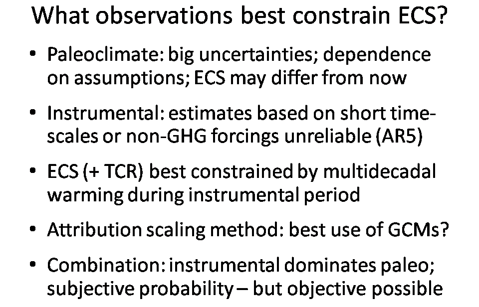
The first three bullet points of Slide 3 reiterate what the IPCC fifth assessment WG1 report (AR5) said in Chapters 10 and 12 about palaeoclimate ECS estimates and those based on short timescales or non-greenhouse gas (GHG) forcings, and its implicit conclusion that estimates based on multidecadal warming during the instrumental period (since about 1850) were likely to prove most reliable and provide the narrowest uncertainty bounds.
ECS estimates based on multidecadal warming typically use simple or intermediate complexity climate models driven by estimated forcing timeseries, and measure how well simulated surface temperatures and ocean heat uptake compare with observations as model parameters are adjusted. Energy budget methods are also used. These involve deriving ECS and/or TCR directly from estimates changes in forcing and measured changes in GMST and ocean heat content, usually between decadal or longer periods at the start and end of the multidecadal analysis period. Alternatively, regression-based slope estimates are sometimes used.
Attribution scaling methods refers to the use of scaling factors (multiple regression coefficients) derived from detection and attribution analyses that match observed warming to the sum of scaled AOGCM responses to different categories of forcing, based on their differing spatiotemporal fingerprints. The derived scaling factor for warming attributable to GHG can then be used to estimate ECS and/or TCR, using a simple model. This hybrid method of observationally-estimating ECS and TCR appears to work better than the ‘PPE’ approach, which involves varying AOGCM model parameters.
Various studies have combined palaeoclimate and instrumental ECS estimates using subjective Bayesian methods. I do not believe that such methods are appropriate for ECS estimation, as the results are sensitive to the subjective choice of prior distribution. It is however possible to use objective methods – both Bayesian and frequentist – to combine probabilistic ECS estimates, provided that the estimates are independent – which palaeo and instrumental estimates are usually assumed to be. However, since palaeo ECS estimates are normally less precise than good instrumental ones, combination estimates are usually dominated by the underlying instrumental estimate.
Slide 4
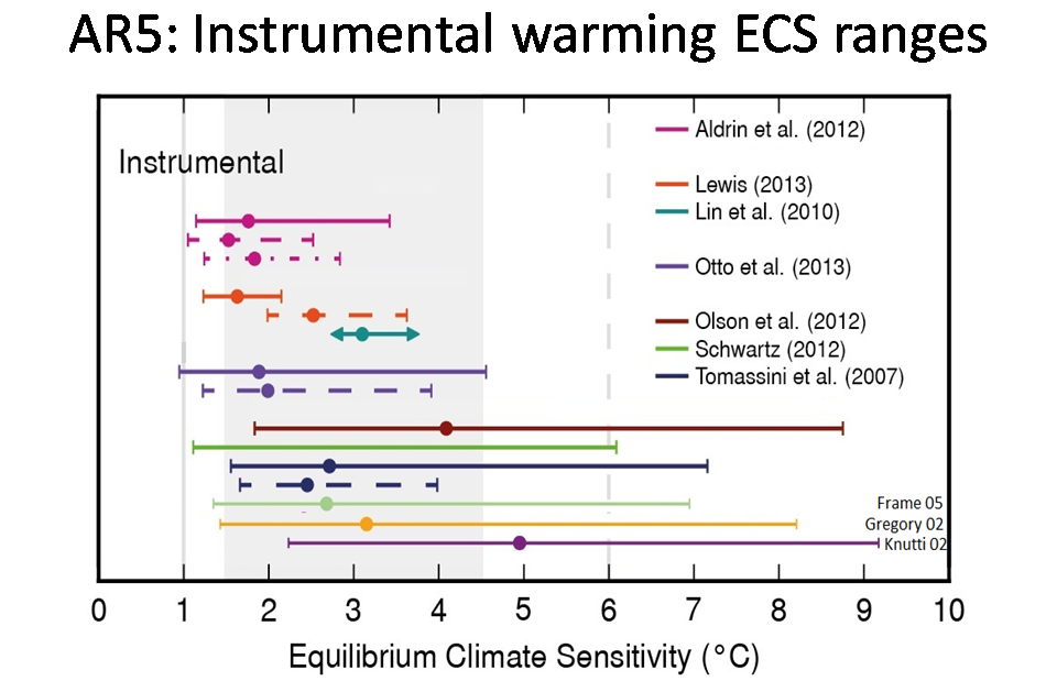
My talk concentrates on ECS estimates based on observed warming observed during the instrumental period, as they are thought to be able to provide the most reliable, best constrained observational estimates. Slide 4 shows a version of Box 12.2, Figure 1 from AR5 with all other types of ECS estimate removed. The bars represent 5–95% uncertainty ranges, with blobs showing the best (median) estimates.
For the Lewis (2013) study, the dashed range should be ignored and the solid range widened to 1.0–3.0°C (with unchanged median) to reflect non-aerosol forcing uncertainty, as discussed in that paper.
Although the underlying forcing and temperature data should be quite similar in all these studies, the estimates vary greatly.
Slide 5

The relevant forcing concept here is ERF, denoted here by ΔF. AR5 defines it as follows: “ERF is the change in net TOA [top of atmosphere] downward radiative flux after allowing for atmospheric temperatures, water vapour and clouds to adjust, but with surface temperature or a portion of surface conditions unchanged.”
ΔT refers to the change in GMST resulting from a change in ERF, and ΔQ to a change in the planetary heating rate, mainly (>90%) reflected in ocean heat uptake.
Without using ocean heat content (OHC) data to estimate ΔQ, ECS tends to be ill-constrained.
ΔQ is not relevant to estimating TCR: the equivalent equation for generic TCR given in AR5 Chapter 10 is TCR = F2xCO2 ⨯ ΔT / ΔF.
Pre-2006 ECS studies almost all used the Levitus (2000) OHC data, which – due apparently to an uncorrected arithmetic error – gave substantially excessive values for ΔQ. Lin 2010 also used an excessive estimate for ΔQ, taken from the primarily model-based Hansen et al (2005) study. Moreover, many of the studies make no allowance for ΔQ being non-negligibly positive at the start of the instrumental period, as the Earth continued its recovery from the Little Ice Age. Gregory et al (2013) gives estimates of steric sea-level rise from 1860 on, derived from a naturally-forced model simulation starting in 850. Converting these to the planetary energy imbalance, and scaling down by 40% to allow for the model ECS of 3°C being high, gives ΔQ values of 0.15 W/m2 over 1860-1880 and 0.2 W/m2 from 1915-1960 (ΔQ being small in the intervening period due to high volcanism).
Multidecadal variability, represented by the quasi-periodic Atlantic Multidecadal Oscillation (AMO) in particular, means that the analysis period chosen is important. The AMO seems to be a genuine internal mode of variability, not as has been argued a forced pattern caused by anthropogenic aerosols.
The NOAA AMO index exhibits 60–70 year cycles over the instrumental period, peaking in the 1870s, around 1940, and in the 2000s. The AMO affects GMST, with a stronger influence in the northern hemisphere. As well as altering heat exchange between the ocean and atmosphere, the AMO also appears to modulate internal forcing through changing clouds – a little recognised point. As I will explain, the AMO can distort ECS estimation more seriously than its influence on GMST – of maybe ~0.2°C peak-to-peak – suggests.
Slide 6
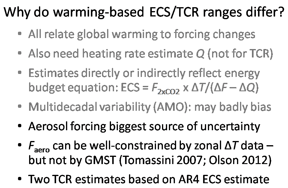
Taking the last point first, the Meinshausen et al (2009) and Rogelj et al (2012) TCR distributions featured in AR5 Figure 10.20(a) as estimated from observational constraints were actually based on ECS distributions selected simply to match the AR4 2-4.5°C ECS range and 3°C best estimate. They should therefore be regarded as estimates based primarily on expert opinion, not observations.
Uncertainty as to the change in aerosol forcing occurring during the instrumental period, ΔFaero, is the most important source of uncertainty in most ECS and TCR estimates based on multidecadal warming. Chapter 8 of AR5 gives a 1.8 W/m2 wide 5-95% range for ΔFaero over 1750–2011, about as large as the best estimate for (ΔF – ΔQ). The Lewis and Curry (2014) energy budget based study used the AR5 best estimate and uncertainty range for aerosol forcing (as well as other forcings), and hence its ECS and TCR estimates have 95% bounds that are much higher than their median values.
Otto et al (2013), although likewise using an energy budget method, used estimated forcings in CMIP5 AOGCMs (Forster et al 2013), which exhibit a narrower uncertainty range than AR5 gives, and adjusted their central value to reflect the difference between AOGCM and AR5 aerosol forcing estimates. Its resulting median estimate for TCR was accordingly almost identical to that in Lewis and Curry (2014), but its 95% bound based on the most recent data was lower.
It is possible to estimate ΔFaero with considerably less uncertainty than that stated in AR5, using “inverse methods” that infer ΔFaero from hemispherically- or zonally-resolved surface temperature data. This takes advantage of the latitudinally-inhomogeneous, northern hemisphere dominated, distribution of anthropogenic aerosol emissions, using a latitudinally-resolving model to estimate the spatial pattern of temperature changes at varying ΔFaero levels. Of the ECS studies featured in AR4 and AR5, Andronova and Schlesinger (2001), Forest et al (2002 and 2006), Liberdoni and Forest (2011/13), Ring, Schlesinger et al (2012), Aldrin et al (2012) and Lewis (2013) used this approach; so did Skeie et al (2014).
However, inverse estimates of ΔFaero are very unreliable if only GMST data is used. At a global level the evolution of ΔFaero and ΔFGHG is very highly correlated (r = 0.98 for the AR5 best estimate timeseries). Moreover, the diverge of the growth rates of the two series post the 1970s, when aerosol emissions flattened out, coincides and gets conflated with the AMO upswing.
Slide 7
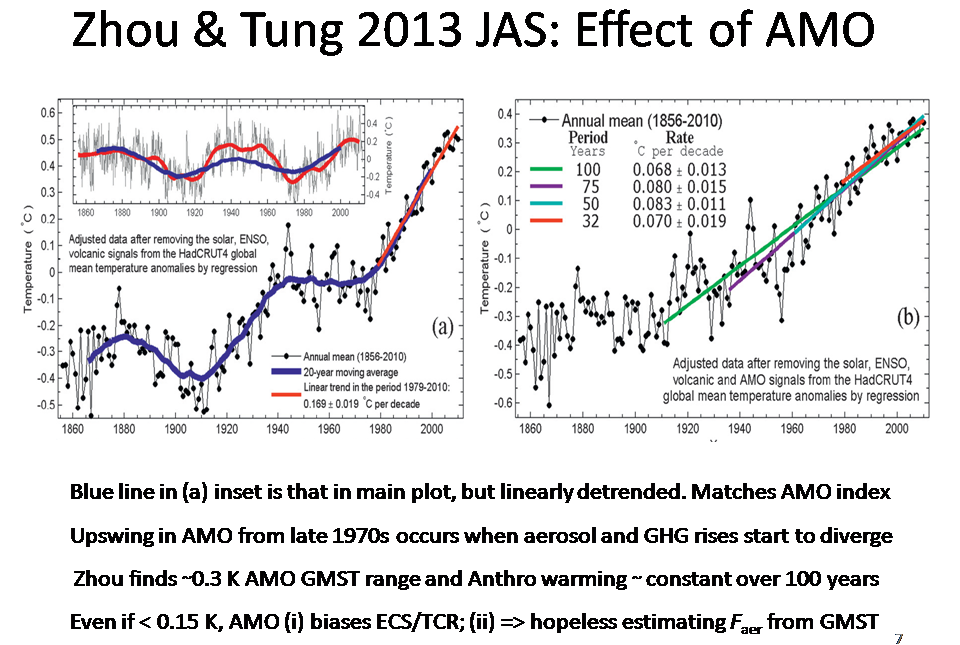
The AMO index smoothed pattern is shown by the red curve in the inset at the top of the LH panel of Slide 7, and can be seen to resemble the detrended GMST with shorter term natural signals removed (blue curve). The RH panel is not relevant to my argument, and can be ignored. Zhou and Tung may be overestimating the influence of the AMO on GMST (their range is in fact over 0.4 K, not 0.3 K as per the slide); Delsole et al (2011) estimate it to be about half as strong. However, even at one-quarter of the level shown it is enough to bias estimation of ΔFaero up by a factor of two or more, with an accompanying upwards bias of 20% or more in the estimate of warming attributable to GHG (and hence in TCR estimates; ECS estimates are even worse affected).
The problem is that a combination of a strongly negative estimate for ΔFaero, and a high estimate for ECS is able to mimic the effect on GMST caused by a factor (the AMO) not represented in the estimation model used. The slight fall in GMST between the 1940s and the early 1970s is matched by selecting a strongly growing negative ΔFaero that counters increasingly positive ΔFGHG, whilst the fast rise in GMST from the late 1970s on is matched by a high ECS (and hence high TCR), operating on a strong rise in ΔFGHG that is no longer countered by strengthening ΔFaero.
The ECS and TCR studies that use only the evolution of GMST (along with data pertaining to ΔQ) to estimate ΔFaero jointly with ECS therefore usually reach a much more negative estimate for ΔFaero, and a higher estimate for ECS, than studies that are able to estimate ΔFaero from the differential evolution of hemispherically- or zonally-resolved surface temperature data. Studies affected by this problem include, for ECS, Knutti et al (2002), Tomassini et al (2007) and Olson et al (2012) and, for TCR, Knutti & Tomassini 2008 and Padilla et al (2011).
Using hemispherically- or zonally-resolved temperature data to estimate aerosol forcing fails to avoid contamination by the AMO when the analysis period is insufficiently long. Many AR4 era ECS and TCR studies used the 20th century as their analysis period. The1900s started with the AMO low and ended with the AMO high. Gillett et al (2012) found that, despite its uses of spatiotemporal patterns, their detection and attribution study’s estimate of warming attributable to GHG was biased ~40% high when based on 1900s data compared to with when the longer 1851-2010 period was used. ECS studies affected by this problem include Gregory et al (2002), Frame et al (2005) and Allen et al (2009).The Stott and Forest (2007) TCR estimate is also affected.
The Gregory and Forster (2008) TCR estimate, while avoiding the AMO’s influence on aerosol forcing estimation, is significantly biased up by the AMO’s direct enhancement of the GMST trend over the short 1970–2006 analysis period used.
I will leave it there for Part 1; in Part 2 I will move on to problems with Bayesian approaches to climate sensitivity estimation.
References
Aldrin, M., M. Holden, P. Guttorp, R.B. Skeie, G. Myhre, and T.K. Berntsen, 2012. Bayesian estimation of climate sensitivity based on a simple climate model fitted to observations of hemispheric temperatures and global ocean heat content. Environmetrics;23: 253–271.
Andronova, N.G. and M.E. Schlesinger, 2001. Objective estimation of the probability density function for climate sensitivity. J. Geophys. Res.,106 (D19): 22605–22611.
DelSole, T., M. K. Tippett, and J. Shukla, 2011: A significant component of unforced multidecadal variability in the recent acceleration of global warming. J. Clim., 24, 909–926.
Forest, C.E., P.H. Stone, A.P. Sokolov, M.R. Allen and M.D. Webster, 2002.Quantifyinguncertainties in climate system properties with the use of recent climate observations. Science; 295: 113–117
Forest, C.E., P.H. Stone and A.P. Sokolov, 2006.EstimatedPDFs of climate system properties including natural and anthropogenic forcings. Geophys. Res. Lett., 33: L01705
Forster, P.M., T. Andrews, P. Good, J.M. Gregory, L.S. Jackson, and M. Zelinka, 2013. Evaluating adjusted forcing and model spread for historical and future scenarios in the CMIP5 generation of climate models. J. Geophys. Res., 118: 1139–1150.
Frame D.J., B.B..B. Booth, J.A. Kettleborough, D.A. Stainforth, J.M. Gregory, M. Collins and M.R. Allen, 2005.Constrainingclimateforecasts: The role of prior assumptions. Geophys. Res. Lett., 32, L09702Fyfe, J.C., N.P. Gillett, and F.W. Zwiers, 2013.Overestimatedglobal warming over the past 20 years. Nature Clim.Ch.; 3.9: 767–769.
Gillett NP, Arora VK, Flato GM, Scinocca JF, von Salzen K (2012) Improved constraints on 21st-century warming derived using 160 years of temperature observations. Geophys. Res. Lett., 39, L01704, doi:10.1029/2011GL050226.
Gregory, J.M., R.J. Stouffer, S.C.B. Raper, P.A. Stott, and N.A. Rayner, 2002. An observationally based estimate of the climate sensitivity. J. Clim.,15: 3117–3121.
Gregory, J. M., and P. M. Forster, 2008: Transient climate response estimated from radiative forcing and observed temperature change. J. Geophys. Res. Atmos., 113, D23105.
Knutti, R., T.F. Stocker, F. Joos, and G.-K. Plattner, 2002. Constraints on radiative forcing and future climate change from observations and climate model ensembles. Nature, 416: 719–723.
Knutti, R., and L. Tomassini, 2008: Constraints on the transient climate response from observed global temperature and ocean heat uptake. Geophys. Res. Lett., 35, L09701.
Levitus, S., J. Antonov, T. Boyer, and C Stephens, 2000. Warming of the world ocean, Science; 287: 5641.2225–2229.
Lewis, N., 2013. An objective Bayesian, improved approach for applying optimal fingerprint techniques to estimate climate sensitivity. J. Clim.,26: 7414–7429.
Lewis N, Curry JA (2014) The implications for climate sensitivity of AR5 forcing and heat uptake estimates. Clim. Dyn. DOI 10.1007/s00382-014-2342-y
Libardoni, A.G. and C. E. Forest, 2011. Sensitivity of distributions of climate system properties to the surface temperature dataset. Geophys. Res. Lett.; 38, L22705. Correction, 2013: doi:10.1002/grl.50480.
Lin, B., et al., 2010: Estimations of climate sensitivity based on top-of-atmosphere radiation imbalance. Atmos. Chem. Phys., 10: 1923–1930.
Meinshausen, M., et al., 2009: Greenhouse-gas emission targets for limiting global warming to 2 °C. Nature, 458, 1158–1162.
Olson, R., R. Sriver, M. Goes, N.M. Urban, H.D. Matthews, M. Haran, and K. Keller, 2012. A climate sensitivity estimate using Bayesian fusion of instrumental observations and an Earth System model. J. Geophys. Res. Atmos.,117: D04103.
Otto, A., et al., 2013. Energy budget constraints on climate response. Nature Geoscience, 6: 415–416.
Padilla, L. E., G. K. Vallis, and C. W. Rowley, 2011: Probabilistic estimates of transient climate sensitivity subject to uncertainty in forcing and natural variability. J. Clim., 24, 5521–5537.
Ring, M.J., D. Lindner, E.F. Cross, and M.E. Schlesinger, 2012. Causes of the global warming observed since the 19th century. Atmos. Clim. Sci., 2: 401–415.
Rogelj, J., M. Meinshausen, and R. Knutti, 2012: Global warming under old and new scenarios using IPCC climate sensitivity range estimates. Nature Clim. Change, 2, 248–253.
Schwartz, S.E., 2012. Determination of Earth’s transient and equilibrium climate sensitivities from observations over the twentieth century: Strong dependence on assumed forcing. Surv.Geophys., 33: 745–777.
Tomassini, L., P. Reichert, R. Knutti, T.F. Stocker, and M.E. Borsuk, 2007. Robust Bayesian uncertainty analysis of climate system properties using Markov chain Monte Carlo methods. J. Clim., 20: 1239–1254.
Zhou, J., and K.-K. Tung, 2013. Deducing multidecadal anthropogenic global warming trends using multiple regression analysis. J. Atmos. Sci., 70, 3–8.


58 Comments
Nicholas:
Thanks for this discussion and elucidation in an area where I have little expertise.
Regarding the estimation of climate sensitivity, I cannot see how a creditable ECS can be attained in view of the general lack of understanding of climate processes.
You hold that the warming shown by the instrumental record of the past 150 years should be the basis of deriving an ECS, which seems a reasonable assertion, but how is it possible to specifically attribute that warming, or any fraction thereof, to increases in atmospheric CO2?
For example, the late warming trend circa 1977-97 has been shown to be due to a decrease in cloud albedo, this decrease due to less cloudiness globally since 1985 (as per public cloud data), hence an increase in insolation which John McLean estimates at 2.5 W/m2 to 5W/m2 (his study was published last year, I think).
Are these sorts of studies ignored by those who derive climate sensitivity figures?
As a further problem, the warming trend circa 1920-1945 started when atmospheric CO2 via man was at 20 ppm, or thereabouts. If you attribute that trend to AGW, do you not have to show an unrealistic CS?. If you do attribute that trend to AGW, how do you support such attribution?
Considerations such as these make all climate sensitivity estimates seem as nothing more than guesswork, and none-too-well informed guesswork, at that.
You say that “the late warming trend circa 1977-97 has been shown to be due to a decrease in cloud albedo” and ask “Are these sorts of studies ignored by those who derive climate sensitivity figures?”
I would say that these sorts of studies typically have less attention paid to them than should be the case, and that too much attention is given by most climate scientists to how globla climate models behave. But there are many studies published, and their findings quite often turn out to have different causes or interpretations than those they put forward.
However, I think it is going a bit far to say that the MCLean study (which I did look at when it came out) has established what you state. Also, decreasing reflection of solar radiation by clouds is one of the mechanisms by which, at least in global climate models, increasing greenhouse gas concentrations cause warming, so the decrease in albedo might not be (wholly) natural.
I think that trying to establish the causes of temperature and other changes over periods of only a few decades is very tricky, due not least to the presence of multidecadal internal variability.
There are sound physical reasons for thinking that rising CO2 wll cause some warming; estimating the magnitude of that effect on the basis of as long a period as practicable, imperfect as it is, seems to me (as it did, I beleive, to the relevant AR5 authors) to be the least bad approach at present.
Nic,
Thanks for your reply. I would be glad to know if any fault in the McLean study, as I was much impressed by it. The study used solid observational data, publicly available, and seemed a very straightforward presentation with no tricks or gimmicks, quite a refreshing experience in this climate thing.
Steve: snip – I ask readers stick to very specific issues of the thread rather than coatracking more general concerns. Nic has provided much to think about here. Please talk about that rather than some other study.
As I remarked here , Andrews et al compute an ECS of 2.1C for the GISS E2-R NINT model based on 150 years of model data while the ECS of the model is 2.7K.
RB
You’ve misread the Schmidt et al 2014 JAMES paper. The ECS of 2.7 C they give is for the Q-flux slab ocean version of GISS-E2-R NINT. The ECS that they estimate for the coupled, dynamic ocean version (which is what is relevant) is 2.3 C, within 10% of the 2.1 C 150-year regression-based estimate.
Thanks Nic. Can you please comment on what differences one might expect between the two alternative measures of transient climate response, namely (1)TCR = response at t=70 years to a forcing sequence of F(t)=1.01^t ⨯ F2xCO2, and (2)TCR = F2xCO2 ⨯ ΔT / ΔF for the actual forcing sequence which we’ve experienced.
HaroldW, Good question. Not much difference, I think.
I carried out some testing on this point for the Lewis and Curry (2014) study and found little difference: see section 2 thereof, just below equation (2). That only dealt with the difference between the formulae used and the profile and duration of the forcing sequence. There is also the issue, raised in Shindell’s 2014 paper and pushed in Gavin Schmidt’s talk at Ringberg, that the transient response to inhomogenous forcing agents, in particular aerosols, might be greater than to CO2. [Hansen’s and Shindell’s earlier work showed that was not the case for the equilibrium response to aerosol, etc, forcing (its efficacy does not exceed one), but that is not relevant here.]
I don’t believe that Shindell’s and Schmidt’s claims of a major bias in TCR estimation are valid, although a bias of a few percent seems possible. I haven’t had access to Gavin Schmidt’s data so I can’t verify his calculations, but I would certainly dispute the values in his penultimate slide. His results are in any case based on a single model (GISS-E2-R) that has a high and unusually made up aerosol forcing. I know of two other models that show the opposite behaviour: they seem to have lower, not higher, transient sensitivity to aerosol forcing than to CO2 forcing. And, ironically, as Gavin Schmidt’s slides show, the GISS-E2-R model has an actual TCR (1.4 C) that is only about 5% higher than observationally-based estimates using an energy budget approach.
FWIW, I second Nic’s opinion here. I have my own model that uses a “stretched exponential” function for the forcing decay curve. I then linearly adjusted the Potsdam AR5 forcing data to match the new aerosol estimates and fit the response function to observed temperatures. I came up with TCR = 1.3C, the same as if I had simply calculated it using ΔT / ΔF.
Thanks Nic. I feel somewhat embarrassed at not remembering that section of L&C. I’ve just downloaded Shindell(2014) and will be reading it this weekend.
I had noticed that the GISS models showed a noticeably smaller ECS for CMIP5, compared to CMIP3, although TCR was little changed.
For CMIP3, the ECS for GISS-EH was 2.7 K and that of GISS-ER 2.7 K.
For CMIP5, the ECS for GISS-E2-H was 2.3 K and that of GISS-E2-R 2.1 K.
TCR: CMIP3 was 1.6 & 1.5 K resp. while CMIP5 was 1.7 & 1.5 K resp.
(CMIP5 per Forster et al./AR5 WG1 Table 9.5; CMIP3 per AR4 WG1 Table 8.2)
Gavin’s Ringberg slide 3 shows GISS-E2-R(TCADI) at ECS=2.4 & TCR=1.6, and GISS-E2-R(NINT) at ECS=2.3 & TCR=1.4. From the graph on slide 4, GISS-E2-H is overshooting badly since 2000, so perhaps GISS is backing away from that version.
Harold,
The CMIP3 vs CMIP5 difference may relate to the slab ocean vs coupled dynamic ocean point – see my response to RB.
Thank you, Nic. Looking forward to Parts 2 and 3.
Cheers
+2
Nic,
I am not sure which approach is more pathetic.
The extended run of a weather forecast model that has 100% errors in two days (without any new observational data insertion – see Sylvie Gravel manuscript ) to century long time periods
in violation of all continuum and discrete mathematical theory.
The simplistic ECS formula that hides all observational data error due to sparsity of sites and instrumental problems, unknown physics
(cloud physics, radiation physics, solar physics, etc.), and nonlinear interactions due to these problems. Then to claim that all of these can be estimated using the questionable observations and/or models.
Gerald, From a mathematical point of view, GCM’s and energy balance methods make unwarranted assumptions. However, my experience with aeronautical fluid flows is that observationally constraining the model is the key. For example, we use boundary layer methods a lot and they are remarkably accurate for many flows. These methods make a number of assumptions that are incorrect, but because they are anchored to lots of data, they often do as well or better than RANS or even LES methods that make fewer theoretical simplifications.
Needless to say, like many, I’ve been learning a lot from Nic on this thread but this was also a very helpful and illuminating comment David, thank you.
Nic, what questions were you asked about this section of your talk. Regards, Steve
Steve,
Apart from a few questions seeking clarification being allowed, questions were after each session of three presentations and, as I recall, not many of those for the session involved were on my talk. Quite a few of the participants seemed more involved in GCM-based investigations than observationally-based work, and maybe some of those people whose studies I had criticised didn’t want to focus on what I had argued. Also, I think most participants believe ECS is at least 2 C and may have not have wanted to focus on observational evidence to the contrary.
I was challenged about the AMO. Some modellers claim that it is forced by aerosols, not natural. But the main attempt to push that argument (by a UK Met Office team, in Booth et al 2012) was demolished by a GFDL team (Zhang et al 2013). I think many modellers are in denial about AMO influence on the rise in GMST since the late 1970s, quite apart from its devasting impact on observational ECS studies that estimate aerosol forcing using only global data.
One participant stated that the anthropogenic warming estimates in the Zhou & Tung study I cited had been shown to be wrong. However, that was not relevant as I was just using their figure to show the correlation between the AMO and multidecadal fluctuations in GMST.
Nic, Thanks for this post. I looked a little at the Ringberg presentations and I didn’t see anything besides your presentation that did a careful job with energy balance models. What in your opinion is the best exposition besides your?
One other thing I noted was that there was a lot about the “inaccuracy” of methods assuming constant feedback factors. What is your thought on this?
David,
The only other Ringberg talk that dealt with similar areas to mine is Gabi Hegerl’s, so it is both the best and the worst other exposition! There are substantial areas of common ground between our talks. I’m happy to discuss any aspects of my talk that conflict with Gabi Hegerl’s. I wouldn’t put any weight on the results of the Schurer et al and Johannason studies she cites until I’ve been able to examine them in detail; their conclusions might not stand up. And I think she has not drawn the right conclusions about the Skeie et al study.
I will deal with the claimed inaccuracy of methods that assume a constant feddback factor in Part 3 of the post, and challenge such claims. As I say at the start of this Part: “Claims that the differences are due to substantial downwards bias in estimates from these observational studies have little support in observations”.
According to a post from Steve Koonin at Judith Curry’s site there isn’t much warming to come from a doubling of co2 levels. And it is bloody difficult to isolate from natural climate variability.
Which is exactly what some of us have been saying for the last 30 years.
Nic,
Thanks once again for a wonderfully enlightening post. You have a way to cut through for people like me that aren’t quite aware of the math and methodology behind many of these papers and explain it concisely. I look forward to part 2. To me it almost seems obvious that the simplicity of the equations alone would never be able to encapsulate the complexity of sensitivity. I am a computer engineer by trade, and a few hobbies including amateur physics interloper, and musician. I enjoy playing in bands at bars and such occasionally, and this reminds me of a discussion we had regarding musicians. Every musician esp in a Jazz band believes themselves to be most important many times, so many have a tendency to showboat, wishing prominence on the bass, trumpet, sax, guitar, vocals, drums, etc…Such prominence given in short periods of time can lead to accurate and worthwhile reflections on the style and music yet…given too much credence, and play, any one part of the whole establishing a long-termed pre-eminence destroys the totality of the music itself. We have a world where sensitivity is estimated assuming the trumpet plays all the solos to begin with, no-one ever hears the other instruments, the melody and harmony are lost, and we end up with naught but trumpeting and preening, while everything else fades, until the music dies. How one could even possibly begin to imagine that ECS can so simply (with such simplistic math) represent all positive and negative factors(the whole symphony) in order to establish one for surety without half the other factors even contributing is beyond comprehension. Without a complete understanding of natural variability and it’s positive and negative correlations to sensitivity, how could one hope to isolate one factor with any remote measure of surety. I apologize if I ramble on or oversimplify and misrepresent.
That solo rambled, but blew a beautiful picture in the air.
============
Thank you DB, Thank you.
I agree that the climate system is very complex, and natural variability causes difficulties in isolating ECS. That is a reason for examining behaviour over a long period during which changes in greenhouse gas forcing are relatively large and decadal and shorter timescale natural variability unimportant, and for seeking to minimise and/or isolate the impact of longer term natural variability.
Despite the complexity of the climate system, it is remarkable how linear, within limits, its behaviour appears to be in terms of simple globally aggregated variables such as GMST, at least according to simulations AOGCMs. CMIP5 models exhibit widely varying ECS and TCR values and the extent and characteristics (and behaviour with warming) of key features such as clouds. Nevertheless, they typically show remarkably linear responses to, for instance, increasing forcing and mixtures of different forcings, changing interhemispherical forcing or temperature contrast, and changes in many other variables scale with the change in GMST.
I note the caveat of linearity within the simulations.
================
Sorry off-topic, but Kloor link left leads to some weird home insurance blog. Recycled site?
Perhaps he didn’t keep up the payments on the URL. 😉
Correct link is http://blogs.discovermagazine.com/collideascape/
Nic,
Thank you again.
1. There seems to be a common assumption that sensitivity of zero should be excluded. This is fairly fundamental because zero would eliminate GHG theory.
Given your persistent work on sensitivity, I assume that you believe that zero is not a possibility. Please correct me if I assume wrongly.
For years I have been trying to find an accepted, mathematical/physical seminal paper that provides a useful, quantitative link between GHG and overall atmospheric temp change (thus not Arrhenius type papers, which do not sample atmospheres).
If you sought to convince me that there was a link between atmospheric temps and GHG concentrations, even one that included which factor was causative of the other, what reference would you provide?
2. I keep hammering the basics in my comments because in my formative years I had to sing “Build on the rock and not upon the sand”. There is still concern that historic temperature trends are not real. For example, I was one of the small team of volunteers looking at Australian temperature data, leading to this Jo Nova post recently.
http://joannenova.com.au/2015/04/two-thirds-of-australias-warming-due-to-adjustments-according-to-84-historic-stations/
Unless or until this study is refuted (and also similar evidence from other countries like the CET records) one has to assume that at least some assumptions in general sensitivity work are badly wrong.
You are doing valuable work which I am not criticising. Simply, I can empathise with the above musician, DB Wood. We are marching to the beats of different drums.
It’s pretty simple.
look at the equation for TCR or ECS.
Steven M
Do you really think that to now I have not read those suppositions?
Think more, write less.
Cheers. Geoff
So explain.. how do those equations take on a value of zero.
Start with climate sensitivity:
lambda = delta T/ delta F
it captures the temperature response to a change in forcing.
do you want to argue that changes in forcing ( like increased or decreased solar input)
will have Zero effect on temperature
perhaps you think that doubling c02 will not increase forcing by 3.7 watts?
a nobel prize awaits you for demonstrating that.
its simple. look at the equation. tell us how it takes on a value of 0
Steven:
I think perhaps Geoff is stating that the net effects of a change in CO2 levels is no change in overall forcing?
that the increase in forcing caused by increases in CO2 is offset by negative feedback mechanisms, so there is no net change in forcing due to changes in CO2?
thats a charitable interpretation of Geoff’s post, one that Im sure you already had knew.
Of course, the pissy, flippant answer to your question is that Lambda is equal to zero when delta T equals zero.
there, FTFY.
snip-
Steve: sorry, these questions have nothing to do with Nic’s post. It is a longstanding blog policy to discourage efforts to prove or disprove general AGW questions in a few sentences or paragraphs or else all threads quickly become identical.
Steven M, I believe Geoff and others are not convinced that all forcing computes as simple as lambda = delta T/ delta F. Bob and Climategrog pointed to the example where the surface handles variance in solar radiation differently than variance in LW. Polar amplification if another postulated effect of GHG. And, if GHG caused excessive fresh water polar melt has even partly the effect on the AMOC that Rahmstorf and Mann claim then there would be significant cooling in the Northern Hemisphere. Since ECS based on direct observation handles all variables, known and unknown, assuming reasonably accurate temperature data, it has a clear advantage over model derivations in this regard.
Nic,
Thank you for this comprehensive overview.
1) Are their any theories on cause of PDO/AMO 60-yr cycle?
2) Do you believe that positive feedback of cloud LW insulation and SW albedo effect just about cancel or the later having more weight?
3) Whereas cloud albedo would seem more effective in the direct sun tropics and cloud LW insulation more effect in the high latitudes, has there attention to this?
4) Are ocean currents believed to vary GMST by varying heat uptake or by a TOA radiative effect caused by effect on equatorial – polar temperature gradient, neither or both?
5) Was there talk of China being a new source of increased aerosol?
6) What is your prediction for the continuation of the pause? Trenberth was just quoted that a “big jump is imminent.”
Was anyone bold enough to voice support to your TCR estimate? Is so, was it publicly or in private confidence?
There was little discussion of TCR at Ringberg. Gavin Schmidt was the only other person that I recall talking about observational estiamtion of TCR, and certainly didn’t support my estimate. But I am in good company with my 1.3-1.4 C TCR estimate. Isaac Held has stated that his personal best estimate of TCR is 1.4 C, and he puts an upper bound of 1.8 C on it IIRC. Isaac is one of the most highly regarded climate scientists. A senior IPCC author likened him (in knowledge) to Yoda.
Do people call Held a lukewarmer?
Richard Drake,
Held says that he thinks TCR is about 1.4, but that ECS is near 3C or higher. He argues that the effective (what Nic calculates from energy balance) is much lower than equilibrium sensitivity, but that will not be evident until century time scales. To which I say: ‘so does it matter at all?’
Isaac Held was elected to the National Academy of Sciences in 2003, has an overwhelming climate bibliography, and addresses his position on climate sensitivity in his 2012 paper, “Constraints on the high end”.
Here is Held’s 2014 paper on TCR from volcanic eruption modeling here. Bottom line is that TCR is modeled 1.1 to 2.6 in CMIP5 but Held shows one can chop off the top half of the range.
Held has some interesting posts at his blog including an old one about simulations of convection showing a lot of sensitivity to the size of the domain. I was surprised a little by his APS climate statement meeting statements which seemed to be less circumspect than most of his blog work.
Yoda’s on the dark side ’til it’s ‘Science of Boon’.
==============
Ron,
Thanks for your comment. I don’t claim to be an expert in all the areas you ask about, but shooting from the hip I would answer as follows:
1) Yes for the AMO; the PDO is a decadal cycle and as such is not a major concern for sensitivity estimation. One physical theory is Dima and Lohmann (2007): A hemispheric mechanism for the Atlantic Multidecadal Oscillation, J Climate (open access). Longer term Pacific variability may be bound up with the AMO, a comprehensive theory being the Wyatt and Curry Stadium wave thesis.
2) I’m not a cloud expert, but if the combined water vapour/lapse rate feedback is as positive as the constant relative humidity thesis (and almost all CMIP5 models) imply, then an ECS of below 2 likely requires net cloud feedback to be negative.
3) Pass.
4) Changing ocean dynamics on a multidecadal timescale (which is of most relevance for sensitivity estimation from on multidecadal warming) seem usually to be regarded as vary GMST by varying heat uptake. But I believe there is good evidence that they also directly vary the TOA balance by affecting clouds. I don’t know if the mechanism involves simply changes in the equatorial – polar temperature gradient.
5) Yes, but the effect seems minor. See Stevens, B. 2015: Rethinking the lower bound on aerosol radiative forcing. J Clim.
6) I’m not one to predict internal variability, but although a resumption of a rising trend would not surprise me, it is unclear to me why a big jump should be imminent. Ocean heat uptake doesn’t seem abnormally high, ESNO is not in a negative phase, and the AMO should be declining, which would partly offset a rising trend due to increasing greenhouse gases.
Several more big pieces just fit into place. I know it’s the edge, and a corner at that, but a picture is coming clear.
===============
Nic
Do you think that its possible that GHG sensitivities might be considerably lower than solar sensitivities for a given forcing. One possible reason for this could be the large difference in water absorption between LWR and SWR.
Bob
It is possible, but I haven’t as yet seen convincing arguments that it is the case. Even if it is the case, that might well mainly imply that sensitivity to solar variations was higher than generally thought, not that sensitivity to GHG variations was lower.
“ΔT refers to the change in GMST resulting from a change in ERF”
How on Earth ( if you’ll forgive the expression ) can one define and energy balance equation based on “average” temperature change of two groups of matter with substancially different heat capacities?
HadCRUFT4 ( sic ) temperature anomalies are area weighted to represent the proportion of land and sea, however they do not account for the difference in heat capacity. This using such a non physical statistical quantity in an energy balance equation is meaningless.
Land near surface air temp changes about twice as fast as SST ( typically taken as MAT proxy ).
Rock has a specific heat capacity about 25% that of water. Most land is not bare rock but “moist” rock. The ratio of 50% shown with BEST land and SST suggests it has a SHC about half that of water.
So takng an arithmetic mean of the two has no physical meaning in terms of energy equations and gives undue weighting to the more rapidly rising land data.
Which, as luck would have it, exaggerates climate sensitivity. But 2,500 of the world’s “top” scientists would not have overlooked something that obvious, would they?
I am going to be as brief as possible with my comments here.
First of all, Nic, I appreciate your posts for being articulate, informative and polite. I look forward to parts 2 and 3.
I have been in the process for some months now downloading all the available CMIP5 model runs and analyzing those data. I have been looking at the RCP scenario, Historical, Historical GHG, Historical Natural, 1% CO2 per year, abrupt 4X CO2 run outputs. My intent was to look for significant differences in model output and to better understand the deterministic part of the CMIP5 model temperature series as represented by TCR and ECS.
My first impression from my analyses was that there are some very different results produced by these models in properties such as decadal internal variability, year to year noise levels and more obviously to those familiar with TCR and ECS model outputs in the deterministic trends due to GHGs. The question here that arises for me is why there is not a serious attempt (of which perhaps I am not aware) by some association of modelers or climate scientists who analyze model outputs to use a criteria for eliminating some of these models at least when looking at model spreads and uncertainties for such values as TRC and ECS?
I have also been surprised that I have been able to find where confidence intervals (CIs) for CMIP5 model TCR values were published. My approach in estimating CIs for TCR values involved obtaining a model for the 1% CO2 model response series and in turn modeling the residuals of that model with an ARMA fit. Using a Monte Carlo approach the estimated 95% CIs ranged from plus/minus 0.14 to plus/minus 0.49 and with an average of 0.23 for 32 CMIP5 models.
Since separating the observed temperature series into the components that produce those series is critical to estimating TCR, I have been wondering as a layperson why more efforts are not published in attempts to reduce these series into the cyclical, white/red noise and deterministic trends parts. Singular Spectrum Analysis (SSA) and Ensemble Empirical Mode Decomposition (EEMD) I would think are under used tools in this area of analysis.
Obviously analyzing the observed temperature series has one disadvantage to the CMIP5 models in that we have only one realization of the observed while with models we can obtain many realizations from multiple runs. Here I would also think, and again as a layperson, that modeling the observed and climate model temperature series would be constructive in more precisely determining the deterministic trends in these series. I was further surprised in looking at the Historical GHG runs for 19 CMIP5 models and how some of those models with multiple runs had widely variable deterministic SSA derived trends even at 55 year time periods.
Kenneth,
Thanks for your comment. I commend your work examining CMIP5 model output. The data has quite a lot of ‘nasties’ in it, but if you have obtained it from KMNI they will probably have dealt with most of them. If you use TOA radiation data, be aware that NCAR have put quite of lot of misprocessed model data in the CMIP5 archive, CESM1-CAM5 rlut output being the worst affected.
As you probably know, CMIP5 was (I understand) open to any group with a model that could perform the required runs and provide the specified output. And the IPCC included all of the CMIP5 models in the ensembles it used, I think partly because of the risk of offending member countries if models were excluded. However, I believe that in their work many climate science modellers do tend to discount models that they think (rightly or wrongly) are poor quality, such as Chinese models (bcc-csm1, BNU-ESM, FGOALS, FIO-ESM) and maybe the Russian model (inmcm4) – although that is actually one of the best performing models in some respects. As you are probably aware, much of the FGOALS-g2 CMIP5 data was withdrawn. I believe that the UK Met Office experts view only three modelling centres as having really decent models, the Met Office naturally being one of them. I’d maybe better not say which the others are.
As you say, there are large differences in the internal interannual, decadal and indeed multidecadal variability between CMIP5 models, both for surface temperature T and net TOA radiation N. I agree that their internal variability makes values for model TCR, at least, somewhat uncertain. ECS values are less affected since they are usually estimated from the abrupt 4x CO2 simulation, where the forcing and hence the changes in T and N are very large. However, the model ECS estimates are uncertain for other reasons.
For those models that have very substantial multidecadal internal variability, it is inevitable that different historical and historicalGHG runs will show significantly different trends even over 55 years. The bcc-csm1-1-m model, for instance, appears to have very strong cyclical multidecadal internal variability.
Keep an eye on inmcm4, the Russian model, which I’ve nicknamed ‘I now may concede maturing 4 models’. It is an outlier among models in three characteristics that I think are very pertinent. And there is a version called 5.
H/t Ron C.
=====
Nic, I am happy to know that someone with a substantial physics and mathematics background and with perhaps a non consensus viewpoint on the matter is familiar as you are with the output of the CMIP5 models. I also want to make a correction to my post above where I stated:
“I have also been surprised that I have been able to find where confidence intervals (CIs) for CMIP5 model TCR values were published.”
Should have been:
I have also been surprised that I have not been able to find where confidence intervals (CIs) for CMIP5 model TCR values were published.
Nic:
This may be surprising to someone with a background in the erratic world of financial statistics. It is less so for anyone with knowledge of engineering and systems analysis.
One of the effects of a negative feedback is to linearise the system, and T^4 is one hell of a strong negative feedback.
However, that does not justify all the endless linear approximations made in M&F2015, where they effectively shunt off the feedback information into the “random” residual.
David Young:
“Held has some interesting posts at his blog including an old one about simulations of convection showing a lot of sensitivity to the size of the domain. I was surprised a little by his APS climate statement meeting statements which seemed to be less circumspect than most of his blog work.”
I do not read at Held’s blog on a regular basis, but I thought his persona was different during the APS climate discussion. He even noted how many years he has been doing climate modeling.
“Climate sensitivity is most reliably estimated from observed warming over the last ~150 years”
Seems to be clear that instrumental is better than paleo – paleo reconstructions are fraught with issues of ‘cherry picking’ based on small number of proxies vs a large, direct and mostly global record in the past century, and imprecision of those proxies. The error bars must be huge, certainly compared with the rather impressive detail we can obtain now measuring global temperature, ocean heat, etc. Not to mention that “ECS may be different from now”, because a different climate will have different sensitivities (albedo, ocean circulation etc.).
My question is whether the ‘IPCC consensus’ is likewise down on paleo-reconstructions? Will they move away from paleo-based or these combined (paleo plus instrumental) estimates and go with instrumental only? If not, why not?
The IPCC AR5 WG1 report is quite downbeat about paleo estimates, and reckons that they only constrain ECS within a 10-90% range of 1-6 C. They authors appear keener on combined paleo-instrumental estiamtes. However, I don’t think they properly understand how Bayesian estimation needs to be applied in such cases. And I’m not sure the realise the extent to which, with reasonably well-constrained instrumental estiamtes, the resulting combination estimates will be dominated by their instrumental components.
Reblogged this on Centinel2012.
11 Trackbacks
[…] Nic Lewis at ClimateAudit: 1st of a 3 part series on his climate sensitivity talk at Ringberg [link] […]
[…] Nic Lewis at ClimateAudit: 1st of a 3 part series on his climate sensitivity talk at Ringberg [link] […]
[…] https://climateaudit.org/2015/04/09/pitfalls-in-climate-sensitivity-estimation-part-1/ […]
[…] « Pitfalls in climate sensitivity estimation: Part 1 […]
[…] Pitfalls in climate sensitivity estimation: Part 1 […]
[…] Pitfalls in climate sensitivity estimation: Part 1 […]
[…] Part 1 I introduced the talk I gave at Ringberg 2015, explained why it focussed on estimation based on […]
[…] Pitfalls in climate sensitivity estimation: Part 1 […]
[…] Pitfalls in climate sensitivity estimation: Part 1 […]
[…] Pitfalls in climate sensitivity estimation: Part 1 […]
[…] los estudios de “sensibilidad climática” vienen de este trabajo de comparación de Nic Lewis: Pitfalls in climate sensitivity estimation: Part 1 Pitfalls in climate sensitivity estimation: Part 2 Y hay algo peor en esta sección de “conducen […]