A guest post by Nicholas Lewis
In Part 1 I introduced the talk I gave at Ringberg 2015, explained why it focussed on estimation based on warming over the instrumental period, and covered problems relating to aerosol forcing and bias caused by the influence of the AMO. I now move on to problems arising when Bayesian probabilistic approaches are used, and then summarize the state of instrumental period warming, observationally-based climate sensitivity estimation as I see it. I explained in Part 1 why other approaches to estimating ECS appear to be less reliable.
Slide 8 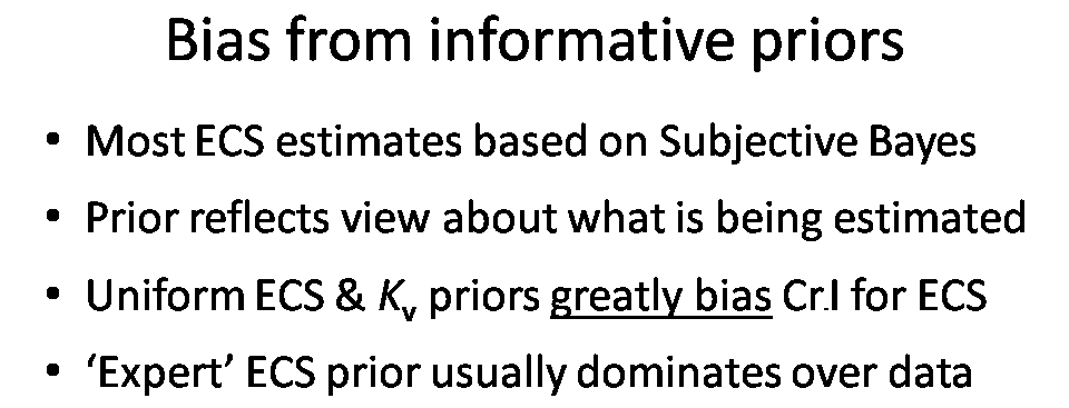
The AR4 report gave probability density functions (PDFs) for all the ECS estimates it presented, and AR5 did so for most of them. PDFs for unknown parameters are a Bayesian probabilistic concept. Under Bayes’ theorem – a variant on the conditional probability lemma – one starts by choosing a prior PDF for the unknown parameter, then multiplies it by the relative probability of having obtained the actual observations at each value of the parameter (the likelihood function), thus obtaining, upon normalising the result to unit total probability, a posterior PDF representing the new estimate of the parameter.
The posterior PDF melds any existing information about the parameter from the prior with information provided by the observations. If multiple parameters are being estimated, a joint prior and a joint likelihood function are required, and marginal posterior PDFs for individual parameters are obtained by integrating out the other parameters from the joint posterior PDF.
Uncertainty ranges derived from percentage points of the integral of the posterior PDF, the posterior cumulative probability distribution (CDF), are known as credible intervals (CrI). The frequentist statistical approach instead gives confidence intervals (CIs), which are conceptually different from CrIs. In general, a Bayesian CrI cannot be exactly equivalent to a frequentist CI no matter what prior is selected. However, for some standard cases they can be the same, and it is typically possible to derive a prior (a probability matching prior) which results in CrIs being close to the corresponding CIs. That is critical if assertions based on a Bayesian CrI are to be true with the promised reliability.
Almost all the PDFs for ECS presented in AR4 and AR5 used a ‘subjective Bayesian’ approach, under which the prior is selected to represent the investigator’s views as to how likely it is the parameter has each possible value. A judgemental or elicited ‘expert prior’ that typically has a peaked distribution indicating a most likely value may be used. Or the prior may be a diffuse, typically uniform, distribution spread over a wide range, intended to convey ignorance and/or with a view to letting the data dominate the posterior PDF. Unfortunately, the fact that a prior is diffuse does not in fact mean that it conveys ignorance or lets the data dominate parameter inference.
AR4 stated that all its PDFs for ECS were presented on a uniform-in-ECS prior basis, although the AR4 authors were mistaken in two cases. In AR5, most ECS PDFs were derived using either uniform or expert priors for ECS (and for other key unknown parameters being estimated alongside ECS).
When the data is weak (is limited and uncertainty is high) the prior can have a major influence on the posterior PDF. Unlike in many areas of physics, that is the situation in climate science, certainly so far as ECS and TCR estimation is concerned. Moreover, the relationships between the principal observable variables (changes in atmospheric and ocean temperatures) and the parameters being estimated – which typically also include ocean effective vertical diffusivity (Kv) when ECS is the target parameter – are highly non-linear.
In these circumstances, use of uniform priors for ECS and Kv (or its square root) greatly biases posterior PDFs for ECS, raising their medians and fattening their upper tails. On the other hand, use of an expert prior typically results in the posterior PDF resembling the prior more than it reflects the data.
Slide 9 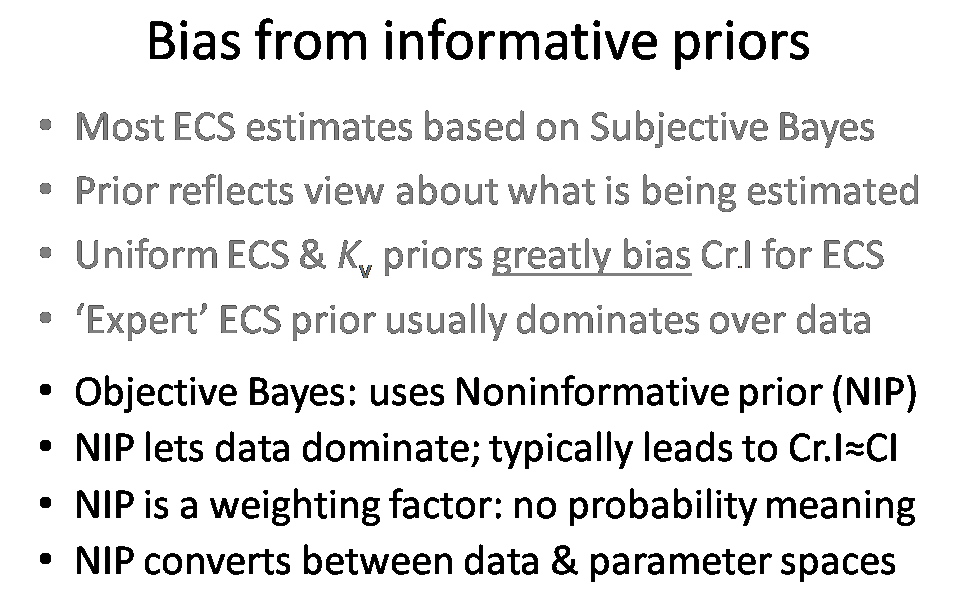
Some studies used, sometimes without realising it, the alternative ‘objective Bayesian’ approach, under which a mathematically-derived noninformative prior is used. Although in most cases it is impossible to formulate a prior that has no influence at all on the posterior PDF, the form of a noninformative prior is calculated so that it allows even weak data to dominate the posterior PDF for the parameter being estimated. Noninformative priors are typically judged by how good the probability-matching properties of the resulting posterior PDFs are.
Noninformative priors do not represent how likely the parameter is to take any particular value and they have no probabilistic interpretation. Noninformative priors are simply weight functions that convert data-based likelihoods into parameter posterior PDFs with desirable characteristics, typically as regards probability matching. This is heresy so far as the currently-dominant Subjective Bayesian school is concerned. In typical ECS and TCR estimation cases, noninformative priors are best regarded as conversion factors between data and parameter spaces.
For readers wanting insight as to why noninformative priors have no probability meaning, contrary to the standard interpretation of Bayes’ theorem, and regarding problems with Bayesian methods generally, I recommend Professor Don Fraser’s writings, perhaps starting with this paper.
The Lewis (2013) and Lewis (2014) studies employed avowedly objective Bayesian approaches, involving noninformative priors. The Andronova and Schlesinger (2001), Gregory et al (2002), Otto et al (2013), and Lewis & Curry (2014) studies all used sampling methods that equated to an objective Bayesian approach. Studies using profile likelihood methods, a frequentist approach that yields approximate CIs, also achieve objective estimation (Allen et al 2009, Lewis 2014).
Slide 10
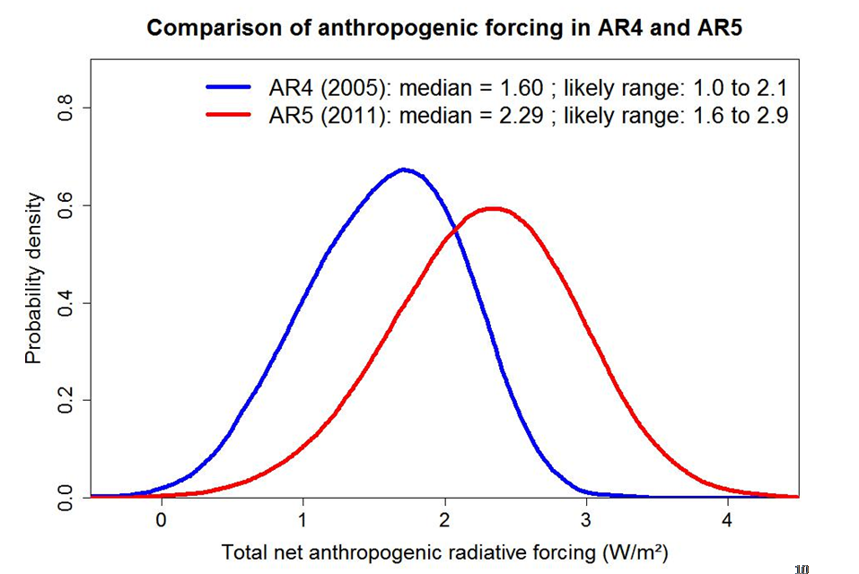
I will illustrate the effect of using a uniform prior for TCR estimation, that being a simpler case than ECS estimation. Slide 10 shows estimated distributions from AR4 and AR5 for anthropogenic forcing, up to respectively 2005 and 2011. These are Bayesian posterior PDFs. They are derived by sampling from estimated uncertainty distributions for each forcing component, and I will assume for the present purposes that they can be considered to be objective.
Slide 11 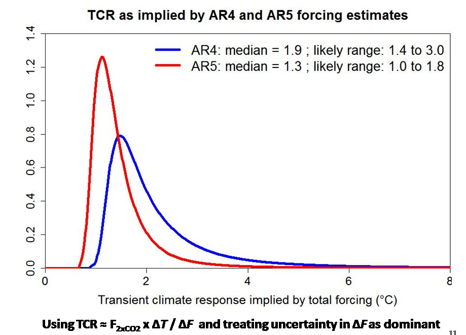
Slide 11 shows posterior PDFs for TCR derived from the AR4 and AR5 PDFs for anthropogenic forcing, ΔF, by making certain simplifying approximations. I have assumed that the generic-TCR formula given in AR5 holds; that uncertainty in the GMST rise attributable to anthropogenic forcing, ΔT , and in F2xCO2, the forcing from a doubling of CO2, is sufficiently small relative to uncertainty in ΔF to be ignored; and that in both cases ΔT = 0.8°C and F2xCO2 = 3.71 W/m2.
On this basis, posterior PDFs for TCR follow from a transformation of variables approach. One simply changes variable from ΔF to TCR (the other factors in the equation being assumed constant). The PDF for TCR at any value TCRa therefore equals the PDF for ΔF at ΔF = F2xCO2 ⨯ ΔT / TCRa , multiplied by the standard Jacobian factor: the absolute derivative of ΔF with respect to TCR at TCRa. That factor equals, up to proportionality, 1/TCR2.
Slide 12 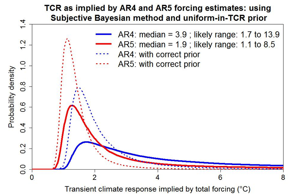
Suppose one regards the posterior PDFs for ΔF as having been derived using uniform priors. This is accurate in so far as components of ΔF have symmetrical uncertainty distributions, but overall it is only an approximation since the most uncertain component, aerosol forcing, is assumed to have an asymmetrical distribution. However, the AR4 and AR5 PDFs for ΔF are not greatly asymmetrical.
On the basis that the posterior PDFs for ΔF correspond to the normalised product of a uniform prior for ΔF and a likelihood function, the PDFs for TCR derived in slide 11 correspond to the normalised product of the same likelihood function (now expressed in terms of TCR) and a prior having the form 1/TCR2. Unlike PDFs, likelihood functions do not depend on which variable that they are expressed in terms of. That is because, unlike a PDF, a likelihood function represents a density for the observed data, not for the variable that it is expressed in terms of.
The solid lines in slide 12 show, on the foregoing basis, what the effect is on the AR4- and AR5-forcing based posterior PDFs for TCR of substituting a uniform-in-TCR prior for the mathematically correct 1/TCR2 prior applying in slide 11 (the PDFs from which are shown dotted). The median (50% probability point), which is the appropriate best estimate to use for a skewed distribution, increases substantially, doubling in the AR4 case. The top of the 17–83% ‘likely’ range more than quadruples in both cases. The distortion for ECS estimates would be even larger.
Slide 12a 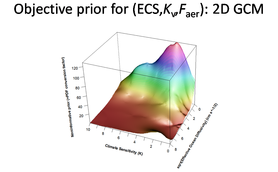
I cut slide 12a out of my talk to shorten it. It shows the computed joint noninformative prior for ECS and sqrt(Kv) from Lewis (2013). Noninformative priors can be quite complex in form when multiple parameters are involved.
Ignore the irregularities and the rise in the front RH corner, which are caused by model noise. Note how steeply the prior falls with sqrt(Kv), which is lowest at the rear, particularly at high ECS levels (towards the left). The value of the prior reflects how informative the data is about the parameters at each point in parameter space. The plot is probability-averaged over all values for aerosol forcing, which was also being estimated. I believe the fact that aerosol forcing is being estimated accounts for the turndown in the prior at low ECS values; when ECS is very low temperaturs change little and the data conveys less information about aerosol forcing.
Slide 13 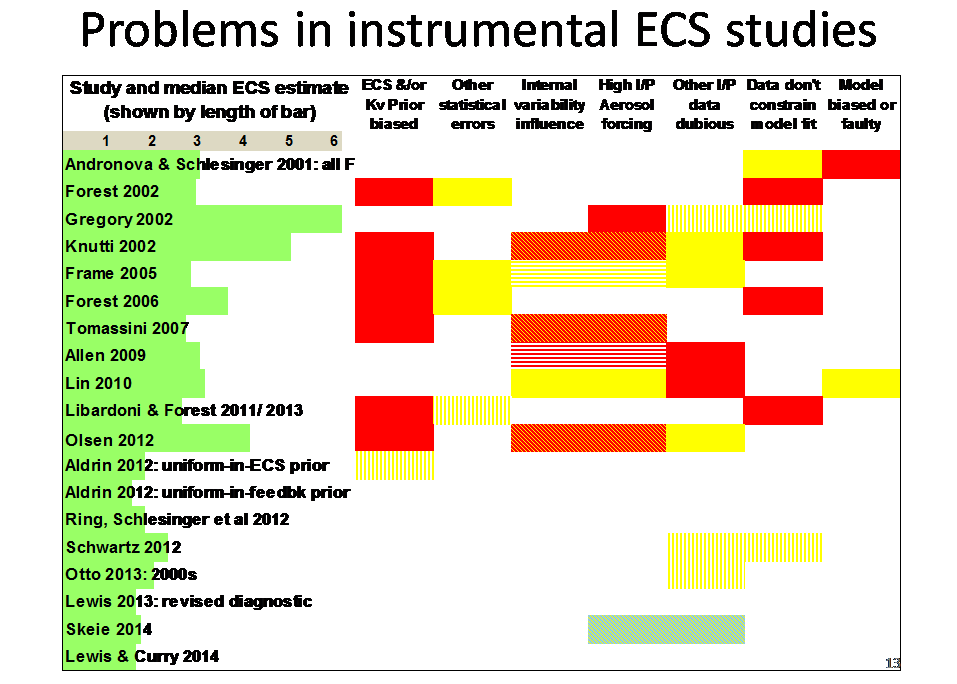
Slide 13 summarises serious problems in instrumental period warming based ECS studies, ordered by year of publication, breaking problems down between seven factors. Median ECS estimates are shown by the green bars at the left.
Blank rectangles imply no significant problem in the area concerned; solid yellow or red rectangles signify respectively a significant and a serious problem; a rectangle with vertical yellow bars, which may look like solid pale yellow, indicates a minor problem.
Red/yellow diagonal bars (may look like a solid orange shade of red) in rectangles across ‘Internal variability influence’ and ‘High input Aerosol forcing’ mean that, due to use of global-only data, internal variability (the AMO) has led to an overly negative estimate for aerosol forcing within the study concerned, and hence to an overestimate of ECS. Yellow or red horizontal bars across those factors for the Frame et al (2005) and Allen et al (2009) studies mean that internal variability appears to have caused respectively significant or serious misestimation of aerosol forcing in the detection and attribution study that was the source of the (GHG-attributable) warming estimate used by the ECS study involved, and hence to upwards bias in that estimate (reflected in a yellow or red rectangle for ‘Other input data dubious’).
The blue/yellow horizontal bar across ‘High input Aerosol forcing’ and ‘Other input data dubious’ for the Skeie et al (2014) study mean that problems in these two areas largely cancelled. Skeie’s method estimated aerosol forcing using hemispherically-resolved model-simulation and observational data. An extremely negative prior for aerosol forcing was used, overlapping so little with the observational data-based likelihood function that the posterior estimate was biased significantly negative. However, the simultaneous use of three ocean heat content observational datasets appears to have led to the negatively biased aerosol forcing being reflected in lower modelled than observed NH warming rather than a higher ECS estimate.
The ‘Data don’t constrain model fit’ red entries for the Forest studies are because, from my experience, warming over the model-simulation run using the claimed best-fit parameter values is substantially greater than per the observational dataset. The same entry for Knutti et al (2002) is because a very weak, pass/fail, statistical test was used in that study.
The ‘Model biased or faulty’ red rectangle for Andronova and Schlesinger (2001) reflects a simple coding error that appears to have significantly biased up its ECS estimation: see Table 3 in Ring et al (2012).
A more detailed analysis of problems with individual ECS studies is available here.
To summarise: all pre-2012 instrumental-period-warming studies had one or more serious problems, and their median ECS estimates varied widely. Most studies from 2012 on do not appear to have serious problems, and their estimates agree quite closely. (The Schwartz 2012 study’s estimate was a composite of five estimates based on different forcing series, the highest ECS estimate comes from a poor quality regression obtained from one of the series.)
Slide 14 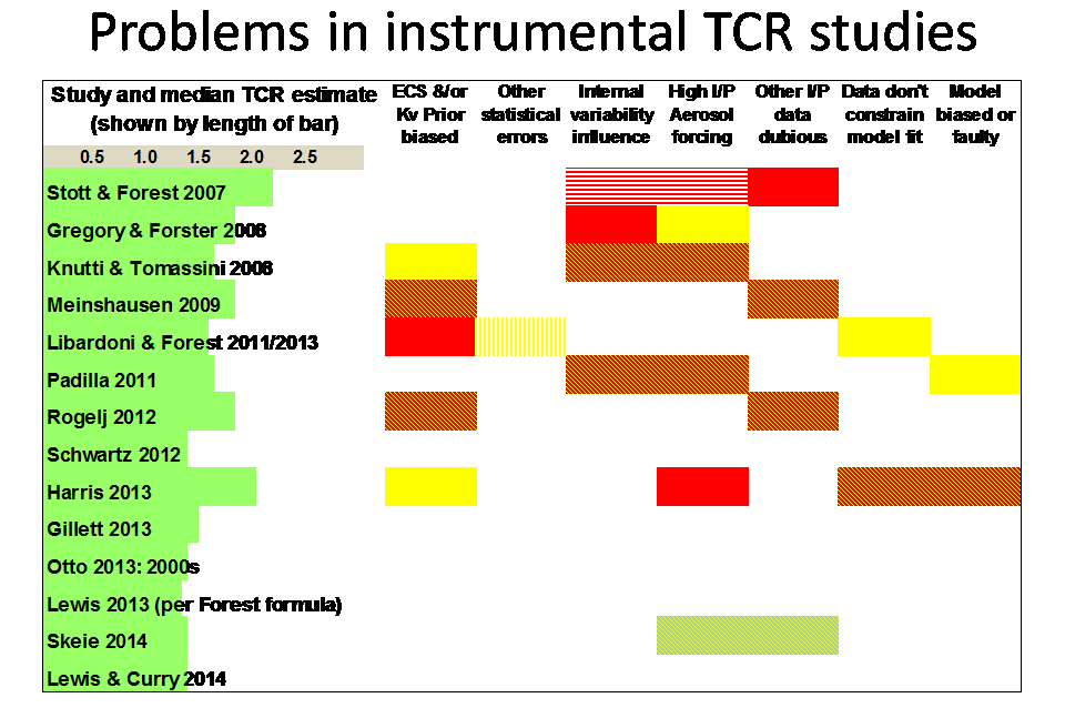
Slide 14 gives similar information to slide 13, but for TCR rather than ECS studies. As for ECS, all pre-2012 studies had one or more serious problems that make their TCR estimates unreliable, whilst most later studies do not have serious problems apparent and their median TCR estimates are quite close to one another.
Rogelj et al (2012)’s high TCR estimate is not genuinely observationally-based; it is derived from an ECS distribution chosen to match the AR4 best estimate and ‘likely’ range for ECS; the same goes for the Meinshausen et al (2009) estimate. The reason for the high TCR estimate from Harris et al (2013) is shown in the next slide.
A more detailed analysis of problems with individual TCR studies is available here.
Slide 14a 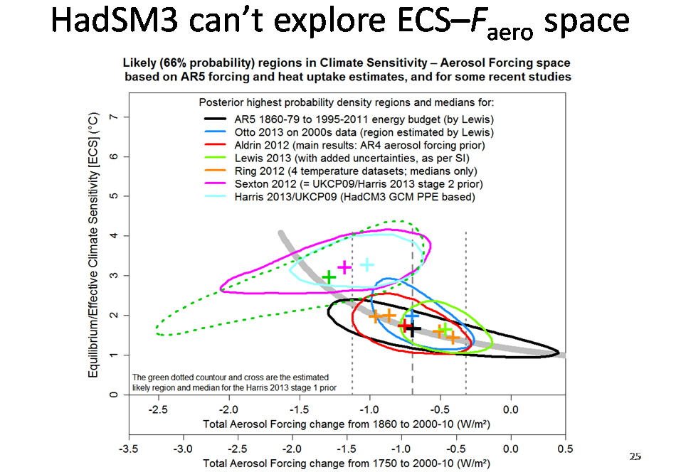
This slide came later in my talk, but rather than defer it to Part 3 I have moved it here as it relates to a PPE (perturbed physics/parameter ensemble) study, Harris et al (2013), mentioned in the previous slide. Although this slide considers ECS estimates, the conclusions reached imply that the Harris et al TCR estimate shown in the previous slide is seriously biased up relative to what observations imply.
The plot is of joint distributions for aerosol forcing and ECS; the solid contours enclose ‘likely’ regions, of highest posterior probability density, containing 66% of total probability. Median estimates are shown by crosses; the four Ring et al (2012) estimates based on different surface temperature datasets are shown separately. The black contour is very close to that for Lewis and Curry (2014).
The grey dashed (dotted) vertical lines show the AR5 median estimate and ‘likely’ range for aerosol forcing, expressed both from 1750 (preindustrial) and from 1860; aerosol forcing in GCMs is normally estimated as the change between 1850 or 1860 and 2000 or 2005. The thick grey curve shows how one might expect the median estimate for ECS using an energy budget approach, based on AR5 non-aerosol forcing best estimates and a realistic estimate for ocean heat uptake, to vary with the estimate used for aerosol forcing.
The median estimates from the studies not using GCMs cluster around the thick grey curve, and their likely regions are orientated along it: under an energy budget or similar model, high ECS estimates are associated with strongly negative aerosol forcing estimates. But the likely regions for the Harris study are orientated very differently, with less negative aerosol forcing being associated with higher, not lower, ECS. Its estimated prior distribution ‘likely’ region (dotted green contour) barely overlaps the posterior regions of the other studies: the study simply does not explore the region of low to moderately negative aerosol forcing, low to moderate ECS which the other studies indicate observations best support. It appears that the HadCM3/SM3 model has structural rigidities that make it unable to explore this region no matter how its key parameters are varied. So it is unsurprising that the Harris et al (2013) estimates for ECS, and hence also for TCR, are high: they cannot be regarded as genuinely observationally-based.
Further information on the problems with the Harris et al (2013) study is available here: see Box 1.
Slide 15 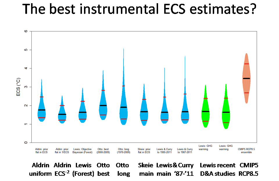
This slide shows what I regard as the least-flawed ECS estimates based on observed warming over the instrumental period, and compares them with ECS values exhibited by the RCP8.5 simulation ensemble of CMIP5 models. I should arguably have included the Schwartz (2012) and Masters (2014) estimates, but I have some concerns about the GCM-derived forcing estimates they use.
The violins span 5–95% ranges; their widths indicate how PDF values vary with ECS. Black lines show medians, red lines span 17–83% ‘likely’ ranges. Published estimates based directly on observed warming are shown in blue. Unpublished estimates of mine based on warming attributable to greenhouse gases inferred by two recent detection and attribution studies are shown in green. CMIP5 models are shown in salmon.
The observational ECS estimates have broadly similar medians and ‘likely’ ranges, all of which are far below the corresponding values for the CMIP5 models.
The ‘Aldrin ECS-2‘ violin is for its estimate that uses a uniform prior for 1/ECS, which equates to a ECS-2 prior for ECS. I believe that to be much closer to a noninformative prior than is the uniform-in-ECS prior used for the main Aldrin et al (2012) results. The Lewis (Forest) estimate is based on the Lewis (2013) preferred main ECS estimate with added non-aerosol forcing uncertainty, as shown in the study’s supplemental information.
Slide 16 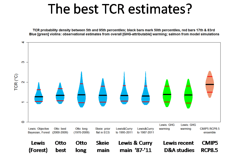
This slide is like the previous one, but relates to TCR not ECS.
As for ECS, the observational TCR estimates have broadly similar medians and ‘likely’ ranges, all of which are well below the corresponding values for the CMIP5 models.
The Schwartz (2012) TCR estimate, which has been omitted for no good reason, has a median of 1.33°C and a 5–95% range of 0.83–2.0°C.
The Lewis (Forest) estimate uses the same formula as in Libardoni and Forest (2011), which also uses the MIT 2D GCM, to derive model TCR from combinations of model ECS and Kv values.
Slide 17 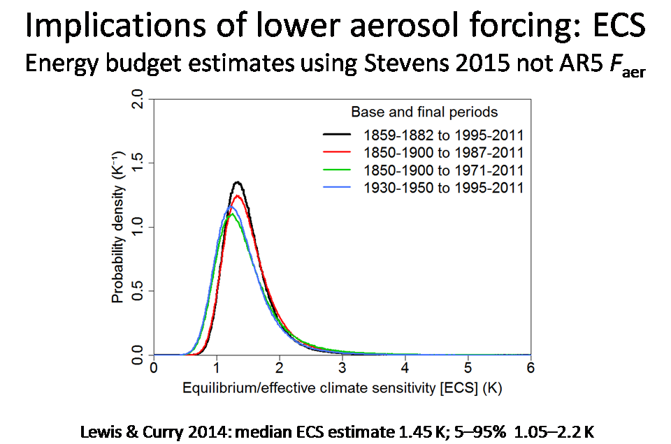
The main cause of long tails in ECS and TCR studies based on observed multidecadal warming is uncertainty as to the strength of aerosol forcing (Faer). I’ll end this part with a pair of slides that show how well constrained the Lewis and Curry (2014) energy-budget main ECS and TCR estimates would be if they were recalculated using the distribution for aerosol forcing implicit in Bjorn Stevens’ recent study instead of the wide AR5 aerosol forcing distribution. (For some reason these slides appear much later, out of order, in the PDF version of my slides on the Ringberg 2015 website.)
The median ECS estimate reduces modestly from 1.64°C to 1.45°C, but the 95% uncertainty bound falls dramatically, from 4.05°C to 2.2°C.
Slide 18 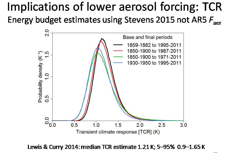
The picture is similar for TCR, although somewhat less dramatic. The median TCR estimate reduces modestly from 1.33°C to 1.21°C, but the 95% uncertainty bound falls much more, from 2.50°C to 1.65°C.
Additional references
Allen MR, Frame DJ, Huntingford C, Jones CD, Lowe JA, Meinshausen M, Meinshausen N (2009) Warming caused by cumulative carbon emissions towards the trillionth tonne. Nature, 458, 1163–6.
Frame DJ, Booth BBB, Kettleborough JA, Stainforth DA, Gregory JM, Collins M, Allen MR (2005) Constraining climate forecasts: The role of prior assumptions. Geophys. Res. Lett., 32, L09702, doi:10.1029/2004GL022241.
Harris, G.R., D.M.H. Sexton, B.B.B. Booth, M. Collins, and J.M. Murphy, 2013. Probabilistic projections of transient climate change. Clim. Dynam., doi:10.1007/s00382–012–1647-y.
Lewis N (2014) Objective Inference for Climate Parameters: Bayesian, Transformation-of-Variables, and Profile Likelihood Approaches. J. Climate, 27, 7270-7284.
Masters T (2014) Observational estimate of climate sensitivity from changes in the rate of ocean heat uptake and comparison to CMIP5 models. Clim Dynam 42:2173-2181 DOI 101007/s00382-013-1770-4
Sexton, D.M. H., J.M. Murphy, M. Collins, and M.J. Webb, 2012. Multivariate probabilistic rojections using imperfect climate models part I: outline of methodology. Clim. Dynam., 38: 2513–2542.
Stevens, B. Rethinking the lower bound on aerosol radiative forcing. In press, J.Clim (2015) doi: http://dx.doi.org/10.1175/JCLI-D-14-00656.1


157 Comments
Great article, though I’d suggest dropping the reference to Fraser’s anti-Bayesian rant. He seems to be arguing that credible intervals aren’t confidence intervals, apparently advocating Fisher’s fiducial statistics. Seriously? Fisher’s one failure?
Drop the Fraser reference paragraph: strengthen and focus your argument.
Lindley proved decades ago that credible intervals can’t in general be confidence intervals. The one dimensional location parameter or transformation of a location parameter case is an exception. Figure 7 in Fraser’s paper that I cited gives a simple illustration in a 2D case of CrIs not being able to match CIs.
I don’t see that Fraser is advocating Fisher’s fiducial statistics (which IIRC requires finding a pivot) as such, although he does deal with confidence distributions, introduced by Fisher. Confidence distributions are coming back into use in quite a big way now.
Don Fraser is certainly more forceful in his critiques of standard Bayesian theory than most statisticians, and not afraid to call a spade a spade. At his age one is allowed to rant a bit! As you may be aware, Don Fraser and his wife Nancy Reid have also done much work in the Bayesian field, developing sophisticated noninformative priors with good probability matching properties.
Yes, it’s well-known that confidence intervals are not credible intervals… except when confidence intervals are plotted on graphs as if they were credible intervals. (Where 100% of non-statisticians and some large proportion of statisticians interpret them as if they were credible intervals.) My question isn’t how he could think they’re different, but why he’s so furious about the distinction that credible intervals are not confidence intervals. (As opposed to the usual confusion that confidence intervals are credible intervals.)
Perhaps he’s arguing that credible intervals aren’t actually credible intervals because priors often aren’t actually prior probabilities. OK, I can understand that. But that doesn’t seem to be his point. If you insist on linking to his paper — which distracts from your main, well-taken points — you might want to link to the discussion replies to his paper:
[1] T. Zhang, “Discussion of ‘Is Bayes Posterior just Quick and Dirty Confidence?’ by D. A. S. Fraser,” Statist. Sci., vol. 26, no. 3, pp. 326–328, Aug. 2011.
[2] Kesar Singh and Minge Xie, “Discussion of ‘Is Bayes Posterior just Quick and Dirty Confidence?’ by D. A. S. Fraser,” Statist. Sci., vol. 26, no. 3, pp. 319-321, Aug. 2011.
[3] Christian P. Robert, “Discussion of ‘Is Bayes Posterior just Quick and Dirty Confidence?’ by D. A. S. Fraser,” Statist. Sci., vol. 26, no. 3, pp. 317-318, Aug. 2011.
It’s Fraser himself who brings up the comparison to Fisher’s fiducial mistake: “.. the function p(θ) can be viewed as a distribution of confidence, as introduced by Fisher (1930) but originally called fiducial…”, as if it were the basis for his argument rather than a failed branch in its lineage.
Again, we’re getting distracted. As far as I can tell, your argument does not depend on a foundational flaw in Bayesian statistics but rather in a naive use of it — in particular priors. Is this not the case?
I agree, we should not get distracted. As you say, my argument does not depend on any foundational flaw in Bayesian theory.
My concern is that there seems to be a misconception amongst climate scientists that priors always have a probability interpretation. So when a prior that varies with 1/ECS^2 is used, it will be perceived as ruling out high ECS values a priori, even if it is in fact a completely noninformative prior. I want readers to realise that this way of thinking is completely wrong.
Don Fraser gives the clearest justification I have seen for noninformative priors having no probabilistic interpretation. Whilst Jose Bernado states that noninformative reference priors have no probabilistic interpretation, he does not give a justification for this statement.
If you wish to give URLs where PDFs of the discussion replies to Don Fraser’s paper can be found (including the supportive reply by Larry Wasserman, and Fraser’s rejoinder), I will attempt to make them into links, although I think that would really be a distraction from the main thrust of my post.
It may have come close to a distraction but that and the previous paragraph shed a lot of light.
Thanks, Nic, for the Fraser reference. It looks like I’ll learn a lot from it. Thanks also to Wayne2 for the additional references. Ditto for them.
Whatever the merits of these arguments, you certainly can’t beat the title of Wasserman’s comment, “Frasian Inference”, his term for Frasier’s advocacy of Bayesian procedures with frequentist validity!
Fraser’s course was the first statistics course that I ever took. We worked off Fraser’s preprints as a text. In retrospect, it was a very strange way to approach statistics as most of us knew math but had no prior knowledge of “ordinary” statistics and no knowledge of Bayes-frequentist disputes.
An interview from 2004 with Donald A.S. Fraser here: http://projecteuclid.org/download/pdfview_1/euclid.ss/1105714168
Steve, were you and your comrades at all challenged by having no independent recourse in the text for material difficult to grasp in the lectures? I was often adrift in a physics course lectured by two guys who were composing a textbook on the subject If I didn’t “get” it in class, what was in the loose-leaf work-in-progress wasn’t going to help.
Reblogged this on Centinel2012.
I second the comments regarding deleting the reference to Fraser. I looked at that reference quickly and I was unable to discern if his criticism was:
(1) with bad priors you get bad posteriors;
(2) if you believe your prior, you can get different results than frequentists do; or
(3) something else.
However, all of us are Bayesians—-some of us admit it but others do not.
See https://xkcd.com/1132/ or
Feynman Lectures on Physics Vol. I, Section 6-3.
It is probably better to realize that the probability concept is in a sense subjective, that it is always based on uncertain knowledge, and that its quantitative evaluation is subject to change as we obtain more information.
Observer
Nic, I also applaud not only your work but the tables, especially the one supplying your opined criticism of the prior studies. That’s a great reference for those of us catching up. I find your trend of TCR/ECS estimations in IPCC reports informative on it’s own. I hope it continues. 🙂
I understand that the PDO/AMO trough in the 1970s could have falsely attributed cooling to aerosols peaking then. But does your ECS/TCR studies weigh for the possibility of PDO/AMO distortion of the temperature record in the 1990s? It did not occur to me until Part II that you only refer the AMO, not the PDO. Why?
Ron, Thanks. The PDO is a decadal cycle and as such is not a major concern for sensitivity estimation. The IPO appears correlated with the SOI/ENSO and it is unclear that it involves a physical mechanism with a cyclical basis, apart from the extent to which it is influenced by the AMO.
Areas influenced by the AMO overlap to a much greater extent with where the increase in aerosol forcing and its flattening off after the 1970s was concentrated than do areas influenced by the PDO/IPO.
Most of the ECS/TCR studies that I consider good use an analysis period covering something like 1860 to some point in the first decade or so of the current century. That pretty much spans two full AMO cycles, so (leving aside the aerosol issue) so the AMO should cause relatively little bias in estimation.
NicL,
How sensitive are these numbers to updated forcing change estimates (e.g. Schmidt et al 2014) and differences in observational datasets used (e.g. BEST/CW2014)?
Also – how do you compensate for the time-lag issue brought up by Ricke et al (2014) with respect to emission versus response?
http://iopscience.iop.org/1748-9326/9/12/124002/article
Final question – when you discuss the AMO – what definition are you using because they differ significantly?
Robert W
Not particularly sensitive. There are many adjustments that one might make to forcing change and observational temperture datasets, based on published research, going in both directions for each. However, I think one should be cautious about doing so. I also think there is a risk that people from modelling centres may tend to look more for adjustments that would bring observationally-based ECS and TCR estimates closer to their, higher, model-based values.
The time-lag between CO2 emission and response brought up by Ricke et al (2014) is obvious and well-known. But surely you can see that it is totally irrelevant when one is estimating ECS and TCR from concentrations not emissions, as in case of all the observationally-based ECS and TCR studies I discuss?
I generally use the NOAA AMO index (Enfield DB, Mestas-Nunez AM, Trimble PJ (2001) The Atlantic multidecadal oscillation and its relationship to rainfall and river flows in the continental US. Geophys Res Lett 28:2077–2080; see http://www.esrl.noaa.gov/psd/data/timeseries/AMO/). It matches closely the Internal Multidecadal Pattern found in Delsole et al (2011) using a quite different method.
Robert,
Given assumptions made by your good self in kriging parts of the Arctic, do you consider that you outcome is good enough to be used in this sensitivity work?
Yes, I am well aware of your work on verification, but I come from a background of geostatistics for ore estimation where one can drill another hole to get more, hopefully better data. There is a financial advantage from getting it right.
The overall outcome is often quite sensitive to the placement in 3D of the boundary between ore and uneconomic mineralisation.
This often puts emphasis on volumes that are at the interpolation/extrapolation crossover and sometimes it involves regard for differnt rock types setting the boundary.
As I read it, C&W does more extrapolation than we would have done; and you seem to pay less attention to boundaries such as sea ice/land ice. So my question is really about whether you consider that your assumptions are robust enough to be used in this sensitivity work, given that you are using guessed values rather than measured, at the extremes.
Geoff
Nic, I meant PMO but 150-yr study spans eliminate bias for that too, thanks.
Has there been any suggestions that TCR is temperature dependent? It seems it would be a nice thing to find out. Is there any thought to the ability to reveal through statistical study, for example, if vapor/cloud-based feedbacks follow a climate temperature curve?
I’m not aware of much evidence that TCR or ECS is materially temperature dependent, within a span from a degree or two colder than now up to four or five degrees warmer, although this is based mainly on model simulations.
Ron and Nic: When thinking about whether ECS should be approximately linear, I find it easier to consider its reciprocal, the climate feedback parameter. After GMST has warmed 1 degC, how much more radiation (OLR and reflected SWR) will be leaving the planet (in W/m2). If the answer is 3.2 W/m2 (net feedback is zero), then ECS (for 2XCO2) is 1.2 degC. If the answer is 1.6 W/m2, then ECS is 2.4 degC. If GMST warms another degC, I expect approximately the same change in OLR and SWR.
This approach to ECS circumvents the details of ocean heat uptake and centuries-long approach to equilibrium. As I see it, OLR and reflected SWR depend only on GMST, not whether ocean heat uptake is large or has ceased. Or, at least this appears to be correct for all fast feedbacks. Ice-albedo feedback from ice cap melting won’t have reached equilibrium.
Things get trickier when you consider how many different ways one can raise GMST by 1 degC: a 1 degC rise everywhere, with polar amplification, more warming in one hemisphere, etc. These possibilities won’t produce exactly the same change in radiation and some are arguing that their isn’t a unique value for ECS for this reason. But there is only one scenario that represents an equilibrium rise of 1 degC in GMST.
Frank, I agree that it is often better to consider the reciprocal of ECS, which is more linearly related to the least well-constrained observable variables.
But there is a big problem with directly estimating the response of TOA radiation to GMST change: it is very difficult to distinguish over the timescales for which data is available between random cloud fluctuations affecting outgoing radiation and thereby causing a change in GMST, and changes in GMST that cause a change in outgoing radiation. Only the second type of effect represents climate feedback. Lindzen, Choi and their colleagues have tried to overcome this problem by using lagged regression, but it is unclear that they have yet succeeded outside the tropics or for SW radiation. I think AR5 was right to express caution about this and other approaches to estimating ECS from short timescale changes.
Ice cap melting is excluded from the definition of ECS, BTW, although sea ice melting and changes in snow cover are included.
Is there anything new in here arising beyond the discussion/debate that occurred a little while back on the ClimateDialogue.org website?
Click to access Climatedialogue.org-extended-summary-climate-sensitivity.pdf
I remember it getting a little impasse-y, and/or not as cut-and-dried as the perspective here (once other experts were in the room discussing).
Yes, there is new material here. But as I didn’t refer to the ClimateDialogue discussions when formulating my Ringberg talk, I couldn’t say how much was covered there.
It would be informative to see the effect of Stevens’ forcing estimates on tcr/ecs on slide 17/18 as a pre-Stevens (ar5) and post-Stevens curve.
The basis period doesn’t seem to change much, so you could thin the number of pdfs down.
(I appreciate that the talk has already been given, but when I got to 17/18 I was scrolling back up to try to see pre-Stevens pdfs to compare.)
Small point: how did you manage to get through all this in the time allowed? There’s an awful lot of material here.
I agree that might have been better. But the comparison of median and 95% estimates provided below the tcr/ecs slides gives most of the important information.
I talked fast, omitted some material and ran slightly out of time!
Outstanding presentation by Judith Curry at US senate hearings absolutely outstanding http://science.house.gov/hearing/full-committee-hearing-president-s-un-climate-pledge-scientifically-justified-or-new-tax
Nic
You say that “But surely you can see that it is totally irrelevant when one is estimating ECS and TCR from concentrations not emissions, as in case of all the observationally-based ECS and TCR studies I discuss”
I understand that this may be the case for TCR but given the inertia in the oceans there is a pretty good phys/chem justification for some lag in the ECS when considering concentration changes. Im not up to speed with your maths and stats, but simple chemistry says there should be a lag component. Am I missing something that your maths already accounts for?
Terry
All studies that estimate ECS from observed warming allow for the lag in temperature response, which is reflected in ocean heat uptake. This is most simply seen from the energy budget equation in slide 5 (Part 1): ECS = F_2xCO2 x ΔT / (ΔF – ΔQ). Here, ΔQ is heat uptake (very largely by the ocean), which is high initially relative to the imposed forcing ΔF (resulting, e.g., from a change in GHG concentrations). This compensates, when applying the formula, for ΔT being low initially.
Nic, If I am understanding ‘subjective Bayesian’ approach it is to mean one must re-evaluate a hypothesis each time a new evidence (analyzed data set) is added to the knowledge base. But in the case of climate science there are so many acting variables hypotheses can be multiple, elastic and even contradictory. Also, with a ‘subjective Bayesian’ approach in which any selected prior can be theoretically recovered by theoretical manipulation of any one of a potpourri of variables, one runs into the Karl Popper dilemma of infallibility. Should there not be a test for validity of a prior by having an established predicted data result criteria set for failure of hypothesis? Would this not automatically require the priors to be weakened and thus give more power to the evidence? For example, if one claims ECS can be above 3.5 should not that require a pre-set establishment of predictions of temperature probability at a given time series, compensated by known frequented events, volcanic eruptions, ENSO shifts, etc…?
Couldn’t find the last Unthreaded post so FYI on Paleo archiving: https://www.authorea.com/users/17200/articles/19163/_show_article
Ron, both subjective and objective Bayesian approaches in principle permit, but do not require, that a new dataset be analysed in the light of all existing quantitative evidence. As you say, doing so would be impracticable in the case of climate science, at least. And it is normal to present the results of a scientific experiment/investigation on a stand-alone basis. Multiple experimental results (analyzed data sets) and then be combined in a meta-analysis.
In an objective Bayesian approach, the general idea is to select a prior that “lets the data speak”, influencing the result as little as possible, rather than conveying any particular view as to what value of the unknown parameter involved is most likely to have. However, one might reasonably truncate such a prior to rule out negative or exceedingly high (say > 10 C) values for ECS, on the basis that the unstable climate system that they imply is not consistent with the history of the planet.
Nic, thanks for your posts. I saw that James Annan commented on the recent Ringberg conference (http://julesandjames.blogspot.com/2015/04/blueskiesresearchorguk-climate.html)
“It’s hard to see how the climate can have changed as we see in the past if the sensitivity to radiative forcing (in its most general sense) was either negligibly low or extremely high.”
I saw you were at the conference as well. Do you agree with him: how low an ECS is “consistent with the history of the planet”?
I agree with James, although we may differ somewhat on what numbers we put forward.
In a paper led by James Annan’s partner Julia Hargreaves, of which he was 2nd author (Hargreaves et al 2012: Can the Last Glacial Maximum constrain climate sensitivity? GRL) an objective regression-based best estimate for ECS of 2.0 C, with a 5-95% range of 0.8-3.6 C, was obtained (this is the estimate that is adjusted for dust). I have no problem with that distribution – ECS estimates based on instrumental-period warming, typically circa 1.6 C, are in its high likelihood region.
I think the true uncertainty of the Hargreaves et al (2012) ECS estimate is probably greater than the 5-95% range implies, however. So, based on that study alone, the 0.8-3.6 C range is probably better regarded as no more than a ‘likely’ (17-83%) range, at best. On the other hand, it seems quite a stretch to make the observed instrumental-period warming consistent with an ECS of below 0.8 C or above 3.6 C, based on which additional evidence it is reasonable IMO to regard that range as 5% and 95% uncertainty bounds.
Nic, what changes, if any, in accepted protocol would you like to see established in the field? For example, I recently found the late Michael Crichton had the same view as myself that any field study undertaken in a politically volatile environment should be done as a tandem exercise of two teams carrying opposing hypotheses reporting their results publicly and simultaneously upon completion. This natural competition would raise the confidence bars not only on the data but on the analysis. The up-front investment cost would be double but the return would pay 10-fold dividends. As it stands now one tribe can safely ignore the other’s ideas but not their votes. A protocol that demands competitive cooperation raises the stock of all.
Ron, I can see merit in Michael Crichton’s and your suggestion, but this is not really my field of expertise.
I enjoy these posts on TCR and ECS, Nic, and particularly ones utilizing Bayesian inferences. I have noted before I am attempting to learn and use it – or at least attempting to find a justification for using it- in my own analyses. It would appear to me that your cases against using uniform or subjective priors in this particular analysis with sparse and uncertain data have been made and yet in the AR5 both of these approaches were used. I know you were an active participant in the AR5 proceedings and I was wondering if you have any comments on how this was rationalized. If one were to question the motivations of the IPCC (and I have and continue to do so to the extent that I judge the IPCC to be acting as a lawyer would in presenting its case in an adversarial court of law, i.e. using evidence that support its case only) uniform and subjective priors will extend the upper probability limits for TCR and ECS. Those upper probability limits are more critical to the argument for drastic and immediate government mitigation of AGW than are the median values – and a point I am certain not lost on those in control at the IPCC. I would guess that with your background and natural curiosity about matters of physics and mathematics you would need no more motivation for your involvement with the IPCC and particularly in the area of TCR and ECS. You have appeared to me to have gone right to root of the issue that has the greatest potential for influencing “informed” policy in tackling the upper probability limits and it is there I am wondering if you were motivated by reasons in addition to scientific curiosity.
Also in the same context there was a comment that I excerpted from the link below that was originally linked above in a Salamano post.
“According to Pueyo the point is that using a reference prior as if it were non-informative “can cause serious trouble unless the amount of data makes the result quite insensitive to the prior, which is rarely the case with climate sensitivity.” and the method of Nic Lewis “results into a vast underestimation of climate sensitivity.”
I believe Pueyo was described as an expert in Bayesian inference, but his last comment would require some extensive knowledge in this area of climate science. Any comments on this exchange.
In addition John Fasullo made some comments in this discussion where it appeared to me he was opposed to ruling out climate models based on lack of conformity to other model and observed results. He also talks about internal variability of climate models preventing a narrowing of the PDF on TCR and ECS. There are large differences in the internal variability for some climate models and that in my mind is sufficient reason to seriously think about developing a criteria for using or not using a model in an ensemble distribution. I think that maintaining a large range of model outcomes, in effect, is having your cake and eating it too, since the large range makes it more difficult to make statements about the observed results falling out of the range or statistically significant probability range of the models, while at the same time allowing a reasonable probability for the higher end of the models’ outputs.
Click to access Climatedialogue.org-extended-summary-climate-sensitivity.pdf
Kenneth –
If one were to consider only GCMs in Bjorn Stevens’ ECS range of 2.0 to 3.5 K (inclusive), it would disqualify 9 of the 23 models whose ECSs are listed in AR5 WG1 Table 9.5. The remaining 14 have an average ECS of 2.7 K (ranging from 2.1 to 3.5), as compared to 3.2 for the entire set of 23, ranging up to 4.7.
Kenneth, Thanks for your comment. Just to clarify, my role in AR5 was as one of the many reviewers, commenting principally on Chapter 10. Frankly, I don’t think any of the climate scientists involved in AR5 has an adequate understanding of Bayesian inference, at least so far as ECS estimation is concerned. This is a criticism of the way climate science and statistical methods have evolved rather than of any particular AR5 author.
I turned my attention to climate sensitivity about four years ago becuase I thought it to be the most important uncertain parameter in climate science, and I soon realised that the use of subjective Bayesian methods with uniform priors in AR4 was completely inapproriate. In my investigations of what approach should be used, I was motivated by pure mathematical/statistical curiosity as well as scientific curiosity and a concern that the risks of climate sensitivity being high were being seriously overstated.
I totally disagree with Pueyo’s claims about reference priors. Read Jose Bernardo’s papers on reference priors, or chapter 5 of Bernardo and Smiths book Bayesian Theory, and judge for yourself. Nor do I agree with Pueyo’s paper about objective priors for ECS.
I’m wary about relying on climate model simulations. But their long preindustrial control runs do provide useful estimates of natural internal variability of the climate system. The ECS and TCR studies that I have been involved with all allow for such variability, based on AOGCM control run data, as do other studies, but it generally does not seem to be the most serious source of uncertainty present.
I would want something more comprehensive including model to model and model to observed comparisons like a ks.test, ARMA model of red noise and standard deviation of white noise. Might be a good time for me to attempt to put a laypersons criteria together for selecting models. I would suppose someone will remind me that a model can get the deterministic part right and the stochastic part wrong. An alternative might be to group the models and then look at ECS and TCR values.
Kenneth, some time ago I tried this approach: http://notrickszone.com/2015/03/05/solar-cycle-weakening-and-german-analysis-shows-climate-models-do-overestimate-co2-forcing/#sthash.B1ipUKjV.Wqps5ViB.dpbs ( see the 2nd part of the post). I ruled out some models with two criteria: 1.: The failures in replicating the trens of observations to 2014; 2. the stability of the model-outputs to 2005 vs. 2014. The resulting TCR of the “good” models was 1.6, for comparison it’s 2.0 of the full ensemble.
Frank, while on a quick look I see that your criteria covers a large range of frequencies, it does use linear trends which I judge to be limiting. Year over year noise is not included nor is auto correlation. If you plot the CMIP5 models temperature series these differences become apparent.
If my criteria resulted TCR values or trends for models higher than expected for the observed that would be informing also.
Kenneth, I’m not sure if autocorrelation is an important thing if one uses 12 month averages just like me, see D/W test ( http://en.wikipedia.org/wiki/Durbin–Watson_statistic ). The “d” is well above one for the trends in this case, so it would surprise me if the autocorrelation had a too big influence on the trends.
Frank, my point on AC of trend residuals – linear or otherwise – was whether a different ARMA model was a better fit for individual models and observed series.
I am looking for ways of distinguishing between these series – and finding a difference with statistical significance.
For my money I’d start by looking at the absolute temperatures they each run at.
Please put me down in the objective Bayesian camp…..let the data do the talking.
Ah, but you see, if the data is mute then the scientist can do the talking.
Objectivity is often just slightly less shameless subjectivity.
Note the recent Planck paper minimizing aerosol uncertainty, pinning it at the minimum, -1.0W/m2…
Nic writes in the post
As I understand that sentence, that’s not correct in most cases, and specifically that’s not correct for the determination of ECS from observations. That cannot be correct, because there are no data-based likelihoods to convert. There’s only one history, and all likelihoods linked to that are model based. Nothing resembling even remotely a frequentist analysis can be even started, when we have only one history rather than an ensemble of identically repeated experiments that lead to a large number of results and allows for counting frequencies.
What the noninformative prior that Nic is using represents is not data based or determined to the least by the data. It’s totally determined by choices made in selecting what data to collect, how to represent the data, the climate model used as a tool in the analysis, and by the way Jeffreys’ rules are applied in fixing the prior. Nothing in the above depends on the data (the climate model used has, however, been influenced by some other observations). Many subjective choices done by scientists involved are included in the process. Nothing is fixed by the system being studied, everything is fixed by subjective choices of people involved.
What Nic is assuming is that the observed temperatures have flat prior distributions. He makes another similar assumption about the ocean flux. These are subjective assumptions about the prior. These assumptions are not dictated or supported by any empirical observations, they are simply Nic’s personal subjective choices. It’s possible that he didn’t know initially where these choices lead. In that respect they differ from typical informative priors, whose consequences are known, when they are chosen, but that does not make Nic’s choices any less subjective or any more objective or any more correct than the expert priors used by others.
What’s a good expert prior is an important question. James Annan has discussed that both in scientific articles and in blog posts a couple of years ago. His preferred choices lead to rather similar final outcome as Nic’s choice. My own favorites are not very different from that, but on detailed level neither Annan’s nor mine subjective preferences are identical with Nic’s choice. It’s unknown, how much the final results would differ from those of Nic. The conclusions are certainly closer to those of Nic than those based a uniform prior in ECS, but that’s about as much I can say about that.
Inferring the PDF or just confidence limits for ECS from a single history is possible only based on the Bayesian approach, and the Bayesian approach is always built on a subjective choice of the prior. Deciding to use Jeffreys’ prior in a specific setting is an equally subjective choice as any of the others, and affects the outcome as much as any other choice that can be considered reasonable at all.
Pekka,
Thank you for your comment. We have some differences in our views on these matters. Probability and statistics has been riven by foundational disputes from early on! It is interesting, however, that your preferred subjective priors are, in the cases involved, not hugely different from what I arrive at using an objective Bayesian approach.
I disagree that there are no “data-based likelihoods” for estimating ECS from observations, but I may be using the term more loosely than you. I accept that the selection of data to use and the uncertainty distributions to attach to the data involves subjectivity. However, I think you will find a considerable commonality or similarity of data used for estimating ECS from observed warming over the instrumental period, so the influence of different choices is typically not that great. And although the uncertainty estimates involve models (to estimate internal variability, for instance), choice of different models typically doesn’t make much difference to the shape of the ECS estimate nor change its median. The width of the ECS estimate distribution is typically dominated by assumptions regarding uncertainty in aerosol forcing.
You say “What Nic is assuming is that the observed temperatures have flat prior distributions.” Effectively, yes, but only because a uniform prior is totally noninformative when errors and other uncertainties in observed temperatures are symmetrical and independent of temperature over the range involved. These are not subjective assumptions by me – they reflect error estimates by the data set providers and the statistical characteristics of internal variability in the AOGCM control runs used to provide estimates of internal variability.
The choice of physical model, to link the variables to which the data used relates with values for ECS and any other unknown parameters being estimated, and the model error assumptions, are also subjective. However, judging from the similarity (when not biased by choice of prior or other faults) of ECS estimates based on similar data but different physical models, extending from single equation energy-budget models to AOGCMs, this is not a critical issue.
Noninformative priors are computed from the likelihood function, and reflect relationships between the data and the model parameters, the assumed data uncertainty distributions and the data values. It is in my view valid to regard them as weight functions, however much that may offend subjective Bayesian purists.
Yes, there is only one history, but that doesn’t mean one has to use a conventional Bayesian approach. One can make multiple draws from the assumed uncertainty distributions to obtain hypothetical realistations if one wishes. That is how Andronova and Schlesinger (2001) derived their PDF for ECS. Or one can use the frequentist profile likelihood method, or more sophisticated developments of it, which provides approximate confidence intervals directly from the likelihood function.
So, yes, of course there is subjectivity in arriving at likelihood function, but they are nevertheless data-based. And to my mind it certainly makes sense to select the prior distribution so as to achieve objective inference (something approximately probability matching) based on the likelihood function used. Why add unnecessary additional subjectivity and likely bias?
Nic,
In my view you mix two issues that are logically independent, while have both a connection to the empirical work.
– The methods of collecting and presenting empirical data.
– The data itself.
The data itself is what tells about the reality.
Your choice of the prior is not at all affected by the data itself, it’s derived from the methods of collecting and presenting data. It’s true that the methods are affected by physical realities, but these realities are realities of doing measurements, not realities of the Earth system. There aren’t any generally valid reasons to think that technicalities of doing measurements form a valid basis for choosing the prior.
It’s, however, true that some priors are extreme in a way that makes them contradict with many different arguments. That’s the case here. You have one approach, James Annan had another, and I have a somewhat different again. We all do, however, deviate from the uniform in ECS in a similar way, because uniform in ECS is rather extreme in it’s own way.
In spite of that agreement all our arguments are purely subjective, supported by some rationale, but subjective anyway. It’s not possible to conclude that those who disagree have made an error or that they are objectively wrong.
Pekka,:
Actually the data tell us absolutely nothing by themselves—they are just numbers in the absence of the context provided by a theoretical framework.
I think this is a pointless distinction. The Universe imposes limitations on how we can collect data for a particular system. Generally it is impossible to completely separate the measurement space from the underlying system we are trying to study.
Whether you do this with statistically based methods or not, regardless you always have to include the measurement method in the model of what you are measuring (and not just what you’d ideally like to have been measuring).
Pekka,
In general, noninformative priors are data-dependent, although many of them, such as Jeffreys’ prior, are not.
Actually the data tell us absolutely nothing by themselves—they are just numbers in the absence of the context provided by a theoretical framework
#####
+100
Now this is interesting. It has always been my assumption that one draws inferences from the data and thus devises theoretical constructs. But now, at this late stage, I am told that this is backwards, that data is meaningless unless it fits some previously devised theory. Or did I misunderstand?
We had a while ago another case, where the idea of non-informative priors was discussed, that related to radiocarbon dating. That was a different case in the way that in that case the “non-informative” prior was very strongly informative in a way that resulted in highly nonsensical results. In the present case, the prior of Nic leads to results that are not highly nonsensical, but the basic problem is still the same.
In both cases the measurements have a variable separating power in the space of model parameters (real age in the radiocarbon case, ECS, ocean diffusivity and aerosols in this case). Nic’s claim is essentially that those regions in the space of model parameters, where the empirical method has little separating power should be given a small weight proportional to the separating power.
In many cases this is justified, but this is not a law that’s true generally; it was not true in the radiocarbon case. It’s necessary to look carefully at the reasons for the low separating power. If it’s due to limitations of the empirical method, it has no value as a guideline in choosing the prior, but when it’s due to the nature of the set of model parameters to be determined, then the low separating power is at least a hint that should be taken into account in choosing the prior.
In the case of radiocarbon dating it was absolutely obvious that the lacking power of the method does not indicate that certain real ages are much less common than both younger and older ages. In this case one part of the effect is related to the fact that a small change in feedback strength has a very large influence for the ECS in the far tail of the ECS PDF. In a model, where feedback strength is considered in some sense a more primary physical parameter than ECS, the prior for the ECS distribution has an rapidly falling tail (inverse square). The relationship between observed temperatures and feedback strength is much more uniform than the relationship between ECS and either one of the others. For this reason my preferences that are based on the idea that feedback strength is more primary than ECS leads to qualitatively similar conclusions than the approach of Nic.
The basic conclusion is that the approach of Nic may give hints about a good choice of prior, but those hints may turn out to totally wrong. Only a more detailed study can tell, what is the more likely conclusion.
Ultimately we are left with a subjective choice, there simply are no objectively favored priors in thew absence of a verified and accepted physical model.
For the record, I disagree with Pekka about the Radiocarbon dating case. The underlying reason why some people, including Pekka, objected to the noninformative prior that I used (Jeffreys’ prior) was that they considered that there was genuine prior information that it did not reflect. Since the study I was critiquing stated that the method used did NOT employ any such prior information, it was appropriate that I did not do so either. Moreover, the prior I used gave results that agreed with the non-Bayesian likelihood ratio methods and perfectly matched frequentist confidence intervals, unlike the prior favoured by Pekka.
Nic,
What makes you think that the way you applied frequentist methods for that case is valid.
You may draw wrong conclusions from misapplying either one of the approaches in that case. That’s a case where common sense works well and proves very clearly thatg your conclusions were not correct even when you agreed that the full PDF cannot be determined but claimed that confidence intervals or credibility intervals can. In reality all these were wrong in a fully obvious way.
In that case common sense is more powerful than erroneously applied statistical methods.
The case was discussed so thoroughly at that time that anyone really interested should check the earlier thread for details.
The problems involved in the term ‘frequentist
statistics’ seem neatly illustrated by this discussion. It was a surprise to me that statistics still uses the term. Taken literally, it precludes most major areas of non-Bayesian applied statistics, viz. econometrics, epidemiology and much besides. There is a marked lack of repeated, exchangeable experiments, let alone attained limits! As too with climate statistics.
Frequentist probability as a universal concept was pretty thoroughly debunked 60+ years ago. Retaining the term seems a recipe for confusion. This is not to say it may not make sense in certain areas of physics where there actually are frequencies which exhibit some long-run convergence. It is also not meant to suggest we should all be subjective Bayesians. There are several ways around frequentist, even if they are non-constructive and semantic. But this is a bit angels and pinheads.
I took a course in Bayesian Statistics from Dennis Lindley many years ago. He tried to convince us to switch to the other side arguing with passion that frequentist probability, and frequentist statistics based on it, are complete rubbish: incoherent, logically flawed, and just the wrong thing to do. But if we still were not convinced, not to worry, because Bayesian and frequentist analyses produce almost the same answers in large samples anyway. I ended up really liking Dr. Lindley but remained a frequentist.
Great discussion going here. From it I would imply that the strict definition of the Bayesian prior defined by some here is that it has to be subjective. I suppose then that the strict Bayesian need only argue about the choice of that prior and how it may affect the posterior – unless we can also argue about the choice of data used. I am not inferring here that the frequentist approach does not have some of the same issues.
Carrick made the point that data is nothing without a theory to connect it to a model and here I see a connection to the choice of the prior for Bayesian inference. If the Bayesian prior is well supported by theory or at least reasonable conjecture then you can call it subjective or whatever and it should take less then comprehensive observed data to make a reasonable inference with the posterior result. With lots of observations the choice of a prior should become less important. The problem I see with many frequentist and Bayesian approaches in climate science is that those using the statistics can misapply or make claims for the results that are not warranted. For me the use of subjective expert priors is particularly troubling in applying Bayesian inference to climate science data.
Kenneth,
Although Carrick made his comment as a protest against something that I had written, I agree fully with Carrick, I had just formulated my thoughts imprecisely.
When frequentist approach is possible and without obvious problems, most people would choose such priors for the Bayesian approach that the results would be similar to the frequentist results. The main difference is that Bayesians think that some conclusions are possible also in cases where frequentist approach is not applicable at all. A genuine frequentist would conclude in those cases that there’s too little data for any conclusions. There are also cases, where the results differ significantly, but in these cases the reasons for that are quite obvious.
Here we are discussing a situation where the frequentist approach cannot be applied as all, because there is far too little data for that.
One way of looking at the prior is to consider it as a measure of the space formed by the parameters being considered. In this measure a range of possible parameter values has a volume that’s proportional to the prior probability that the true value is within this range. The fundamental problem is that mathematics cannot tell, what is the preferred measure in a space spanned by continuous parameters.
When we are looking at physical systems, physics can in some cases tell that. To take an example we may consider a single particle moving freely in space. In this case physics tells that the measure is proportional to the ordinary concept of volume multiplied by the volume calculated from components of linear momentum (or velocity). This rule for calculating the measure leads to the ordinary kinetic gas theory that has been found to be valid for nearly ideal gases. It’s, however, not totally obvious that the linear momentum is one of the natural variables rather than some power of it or something else.
When we move to more complex situations like ECS or the empirical observables used in determining ECS, it’s not to the least clear, what are the natural variables that can be used in a linear fashion in the analysis. It’s not obvious, because we do not have any comprehensive enough physical theory to tell that. Furthermore we have practically no empirical data that would help in deciding on that. The best that we have are some crude theoretical ideas related to our present understanding of the Earth system. One of these ideas is that the model based on the concept of feedbacks might be an applicable approximation and that the feedback strength might be a variable that could be assumed to have a rather uniform probability measure over the relevant range. That’s my preference, and I have told in an earlier comment, where that leads.
What is directly measurable is in many cases also a quantity that might be expected to have an uniform natural probability density, but there are innumerable exceptions to that (the case of radiocarbon dating is a good example).
When we are looking at physical systems and when we are doing empirical work on them, we do always have at least some limited understanding of relationships between variables. That means that we have some information as basis for choosing the priors. We do have information on the empirical methods and we do have information on the data handling. This information must be taken into account, when we are looking at a prior that can be considered uninformative on the physical parameters we are trying to determine.
If we know that very many real world situations lead to a similar outcome in the empirical data while a fraction of possible situations leads to significantly different empirical observations, it would be highly informative in a wrong way to take a prior that’s uniform in empirical values. That kind of erroneous assumption was behind the nonsensical results in the case of radiocarbon dating.
In this case we can tell that the choices of Nic led to a highly informative prior as shown in his slide 12a. That’s not uniformative, that’s highly informative for the determination of ECS. The same reason that I have discussed above is part of that, but we do not really understand what else is there. The fact that we understand only part of the mechanisms that lead to that highly informative outcome does not make the prior any less informative, it’s just informative in an unknown way. Deciding to use such a highly informative prior is a subjective choice that cannot be justified objectively.
I do certainly prefer informative priors whose basis is understood over informative priors whose basis is badly understood, and impossible to justify by known physical arguments. For this reason I dislike strongly Nic’s choice. It includes some strong potential distortions whose nature is unknown.
Pekka,
You write “In this case we can tell that the choices of Nic led to a highly informative prior as shown in his slide 12a. That’s not uniformative, that’s highly informative for the determination of ECS.”
You are mistaken. On the basis that the ‘optimal fingerprint’ based whitening preprocessing of the observational data is valid, that prior is noninformative for the estimation of the joint posterior PDF for ECS, sqrt(ocean effective vertical diffusivity) and aerosol forcing. And it is virtually noninformative for the estiamtion of a marginal posterior PDF for ECS.
I can say that because the whitening is designed to produce independent standard normal variables, for estiamtion of which uniform priors are known to be completely noninformative. Applying uniform priors to the joint likelihood function gives a joint posterior distribution for the true value of the whitened observables. The 3D PDF of which slide 12a shows a 2D marginal version is simply the Jacobian determinant for the dimensionally-reducing transformation of variables from whitened observables space to parameter space.
I arrive at an almost identical marginal distribution (in this case a confidence distribution) for ECS by using a standard frequentist profile likelihood method.
I do agree with you that concepts of measure are highly relevant here. Maybe you are unaware that this is a key concept underlying the Jeffreys’ prior.
Nic,
You pick your in a subjectice way your criteria to prove that you have a noninformative prior, but that’s a fully circular argument.
It’s a simple well known fact that there are no objectively noninformative priors for problems based on continuous variables. That has been accepted also by many well known experts who favor the use of rule-based priors like Jeffreys’ prior as a practical solution, when it’s more important to remove intentional bias that to get results that are most likely to be correct.
Pekka,
What you say is an overgeneralisation. Where the continuous variable parameter involved is a location parameter, a uniform prior is completely noninformative: that is the exception to the general rule, and it extends to transformations of a location parameter.
Agreement between the Bayesian posterior PDFs I obtain and confidence distrbutions obtained using a frequentist profile likelihood method doesn’t strike me as a subjective criteria.
Nic,
It’s not. Only in systems that are controlled by a well verified theory can we tell, what’s a “location parameter” in the sense that a uniform distribution is objectively correct, and even then only, when no additional information changes that. in practice that’s extremely seldom true.
Where is your agreement between a frequentist profile that you compare with results obtained from some particular prior?
None of the cases that have been discussed here provides any frequentist profile to compare with. The data that could show that is missing and it’s impossible to collect such data in these cases.
Thank you to Nic, Pekka and Ken for this discussion.
Nic:
Is this a sufficient reason not to use an expert-elicited prior for this particular case?
As I understand it, the prior distribution should, ideally, be the best representation of our knowledge at the time of the introduction of the new data. We now have good reason to believe that we have a reasonable idea of the likely range within which modern transient & effective climate sensitivity lie, so it’s not clear to me why a non-informative prior is required. (This might just be due to my limited grasp of the topic).
Per Mosher, I’d prefer to see the results for a set of competing priors, and then perhaps a discussion of which is best.
oneuniverse
It is normal to report estimates of unknown variables derived from a scientific experiment on the basis of knowledge gained from that experiment alone. Information gained from different experiments can then be pooled through metastudies or, qualitatively, in review studies (of which IPCC assessment reports are an example).
Thanks Nic, I had mistakenly thought that you were using the Jeffreys prior to immediately derive a posterior which represented our best estimate of ECS in general.
By the way, is there an established mathematical framework for gathering into a single Bayesian assessment the various observational studies of what is by necessity a single climate experiment ? It seems like a difficult problem.
Oneuniverse,
To the extent various empirical studies are independent they can be considered successively. First study modifies the original prior to first posterior distribution. Then this is used as prior for the next analysis, etc. The steps commute, i.e., the final outcome does not depend on the order the studies are considered.
In practice the studies are often not independent. In that case it’s difficult to combine them correctly as the common part tends to be counted many times, which distorts the outcome.
oneuniverse,
There have been various proposals for doing so, e.g. the Bayesian Melding Approach. I have proposed an objective Bayesian approach that derives a noninformative prior for inference from all the available observational evidence, provided it is independent. That method is commutative, and for ECS studies at least gives results that agree with frequentist profile likelihood methods. I don’t recommend the standard subjective Bayesian approach that Pekka mentions, unless the likelihood functions for the two studies have similar forms.
As Pekka says, correctly combining evidence from non-independent studies is difficult. So it is probably OK to combine the results of an insrumental period study with a paleocliamte study (maybe more than one, if from different past periods), but not results from two studies dependent on observed warming during the isntrumental period.
Nic
You are not deriving anything about your prior from observational evidence.
You are deriving everything that affects the prior from the way the measurements have been set up and analyzed, i.e. from the methodological choices, not from the results that have been obtained.
It’s actually good that the data does not affect the prior, because it were not a prior if it were affected by data. There were also a major risk of double-counting in that case.
“As Pekka says, correctly combining evidence from non-independent studies is difficult. So it is probably OK to combine the results of an insrumental period study with a paleocliamte study (maybe more than one, if from different past periods), but not results from two studies dependent on observed warming during the isntrumental period.”
How would independence of instrumental and paleoclimate studies be reconciled with the selection criteria for the proxies for paleoclimate temperature reconstructions that invariably is based (directly or indirectly) on how well the response correlates with the instrumental record? A method whereby the proxy selection criteria is developed using reasonable physical bases prior to selection and then using all the proxy data would provide a more independent basis – or could also show that the proxy response did not have a reasonable temperature signal.
Nic, Pekka, Ken, thank you for the explanation and references.
Nic, might it be possible to place the full text of Lewis 2013 online (or even to provide me with a copy) ?
I’m finding the lecture notes from Prof. Michael Jordan’s stats course useful. This is from lecture 7, as it seems relevant :
Oneuniverse,
What Michael Jordan writes does not help in resolving the question we have discussed. He refers to Jeffreys’ prior, but there’s an infinity of Jeffreys’ priors, because any nonlinear transformation of the variable results in another Jeffreys’ prior, and because we have been arguing on issues linked directly to different variables or sets of variables that are related in a non-linear way.
What makes this case so difficult is that there are many competing alternatives for the variables including ECS itself and the feedback coefficient as well as the complex set of parameters that Nic wants to use.
Pekka, no, I didn’t think it resolved your discussion with Nic, it just clarified the idea behind the ‘noninformative’ prior a bit for me. (I don’t find the term ‘objective bayesian’ a very helpful one in this debate by the way).
I’m not sure I can yet see how aiming to pick a prior that maximizes the divergence between prior & posterior actually ‘let’s the data speak for itself’. Intuitively, I can see an argument (flawed I think) that, since there is a certain distance to be travelled before a prior, through many updates, converges on a good “truthful” posterior distribution (making the particular choice of prior irrelevant), then picking an initial prior that maximises the distance travelled on the first update is a good first step, as it were. However, this isn’t the case if the maximisation occurs because the prior is way off-base, and the non-informative prior cannot provide any guarantees of that, no more than an expert prior can.
In fact, the “ideal” prior could be argued to be the one that is, oracularly, already as close as possible to the “truthful” (unknown final) posterior distribution. ie. that could be an argument that we should be aiming to minimize the divergence between prior and posterior. (I don’t think this argument works in general either).
Nic, I just saw the link to your website & papers, thank you – sorry I missed it. (Google Scholar has missed it too btw)
Oneuniverse,
Waking up in new morning I think that your excerpt may, indeed, help in understanding, why Nic disagrees with my thinking (or vice versa).
Let’s consider another problem. Someone has developed a new empirical method and the question is presented:
What are the cases where the new method is most useful?
It’s obvious that it’s not useful to measure inaccurately a quantity that’s already well known. As an example radiocarbon dating is of little value, if it’s already known that the age of a sample is between 1100 and 1170 years, because all ages in that interval result in essentially the same radiocarbon age, but it may be useful, if we know already that the age is between 1260 and 1330 years, because the radiocarbon age changes monotonically and rather uniformly by almost 200 years over this range of real age.
When we presented the more specific question:
What is the prior knowledge that makes this method maximally useful?
we may derive a prior that is “uninformative” in a very specific technical sense. It allows the new method add maximally to the knowledge. It might be call maximally uninformative with respect to that specific method.
Your pseudonym tells, why this cannot be used as a widely valid basis for choosing the prior. We live in one universe. Our prior knowledge is prior in that one universe. Our prior knowledge does not change, when a new empirical method is developed, but has not been used yet. We cannot jump from one prior knowledge to another when we switch from planning to use one empirical method to planning to use another.
It is true that it’s common that the things that can be measured well are more important than things that are more difficult to measure, but that’s only common, not a law of nature. Such a rule is not valid so well that it could be a good basis for choosing our prior, when we are searching for an uninformative prior in a more general sense than as allowing maximal value for a specific empirical method.
When we let the properties of a method with all it’s weaknesses to dominate our thinking, we end up with such absurd results as those of Doug Keenan on radiocarbon dating. Nobody can tell, how badly Nic’s method of determining ECS distorts his results as nobody has studied his method or his prior in a way that would tell about that. What I can continue to say is that there’s no objective basis for concluding that his method leads to an uninformative prior for the general question of determining the value of ECS in the one universe we live in.
Nic’s slide 12a tells about the separating power of his method in different parts of the parameter space. As discussed above, this has at best marginal value as an indicator of uninformative prior likelihoods of various points in the parameter space. It’s not totally accidental that my preferred subjective prior has some similarity with that, but that’s as much as I’m ready to accept: Some similarity with reasonable subjective priors justified by physics based arguments.
Good morning Pekka,
I think everyone acknowledges that the Jeffreys and reference priors are dependent on the experimental framing of the observed events (and thus in violation the likelihood principle), and I don’t think that Nic is arguing that a particular method of ‘objectively’ generating a prior will always provide the best results, or even that ‘objective’ priors are always to be preferred. However, it seems that there are situations where such priors turn out to be good choices, and not just by accident.
Nic makes a specific argument in Lewis 2013 for his use of the prior in slide 12a. I have a fair bit of back-reading and working through examples to do if I’m to be in a position to assess it, but I don’t think it can be rejected from just the general ‘subjective’ Bayesian objections to it that you’ve raised here (apologies if I’ve missed more specific ones).
I still think that a well-elicited expert prior is to be preferred when attempting to come up with a general best estimate (as opposed to the single-study result that Nic was aiming) and when we do have some prior knowledge of the subject, and the new evidence is weak. Just a layman’s opinion though, and I hold on to it lightly.
By the way, what is your preferred prior that you mentioned ?
Oneuniverse,
My preference for prior is not fully fixed, but my view of the physical situation is that the feedback strength is largely determined by independent factors in a way that makes the prior relatively flat for the feedback strength. All high climate sensitivities correspond to a feedback coefficient close to 1.0 (just below 1.0) which makes their combined likelihood limited. As the high climate sensitivities form the unlimited high tail of the ECS distribution, the tail must be cut off effectively. The most natural form for that cut off seems to be the inverse square, but the cutoff might be slightly slower or even much stronger.
There’s, however, one caveat. In that approach the point of singularity at 1.0 in feedback parameter is not an obvious upper limit. Thus the model includes the (prior) possibility of instability – a real tipping point at feedback parameter of 1.0. The theoretical argument alone cannot exclude that possibility, to do that we must rely on the historical observation that the Earth system has not shown signs of being unstable in that way (again one more caveat: the glacial cycles might be interpreted to indicate such instability over a limited range of state of the Earth system).
Oneuniverse:
“I still think that a well-elicited expert prior is to be preferred when attempting to come up with a general best estimate (as opposed to the single-study result that Nic was aiming) and when we do have some prior knowledge of the subject, and the new evidence is weak. Just a layman’s opinion though, and I hold on to it lightly.”
In the case of TCR or ECS from where would the expert prior derive? From model estimates?
In my mind using a Bayesian inference with an expert prior in combination with sparse and variable observed data would merely lend undeserved credence to a consensus that is not necessarily supported by solid observations. I think this would be a case where Bayesian inference is abused.
Kenneth,
The problem is that there really are no alternatives for Bayesian inference.
We can either pick some prior and get some estimates or conclude that the data is not sufficient for telling anything about the uncertainty range.
Frequentist approach would require much more data even if it were accepted as an alternative.
Pekka, many thanks for the explanation.
Kenneth, I was thinking of a best-effort prior primarily based on observations and existing knowledge of nature, with limitations of knowledge represented by a partial noninformative character to the prior imparted according to best practices of objective bayesian analysis. Perhaps this isn’t realistic.
If the new data is at odds with any consensus represented by the prior, the posterior will represent a diminished or dispersed credence in that consensus, weaker data having less of an impact, as it should. I agree about the potential for bias and abuse, as happened with the IPCC AR4’s imposition of uniform ECS priors with unreasonably high ranges, highlighted in detail by Nic. Subjective or objective, the quality of the posterior relies on that of the prior being good when the data is sparse. (The quality of the objective prior seems to depend on the appropriateness of the chosen statistical model.)
re: subjective vs objective
I came across this brief paper, if it’s of interest – “The Case for Objective Bayesian Analysis” (Berger 2006)
Pekka
“You are not deriving anything about your prior from observational evidence.”
You misunderstood what I wrote, being:
“I have proposed an objective Bayesian approach that derives a noninformative prior for inference from all the available observational evidence”.
I meant here that all the available observational evidence is used for inference (about the unknown parameters), not that all the available observational evidence is used to derive the noninformative prior. Admittedly, the wording could have been clearer.
Nic,
I don’t understand your latest comment. It’s basic in all Bayesian inference that all available observational evidence can by used in succession. There’s the big caveat that it’s very difficult to simultaneously include all information and avoid double counting. No specific prior is any better in that sense than any other reasonable priors (some priors may be worse by effectively excluding important parts of the parameter space).
I can’t see in your work any additional progress in resolving the problems that make combining partly dependent empirical analyses, neither do I see anything else that would further work in that direction.
What I see are unsupported claims about the inferiority of the approaches others have taken.
The discussion with Oneuniverse and the links he has provided has confirmed and somewhat clarified my earlier thinking:
Jeffreys’ prior tells where the particular method has separating power. That may be correlated with what’s likely with minimal prior knowledge, but that’s only a possibility, not a law of nature or statistics. (The case of radiocarbon dating is a certain failure of that expectation.) How much correlation there’s in the case of ECS determination can be studied, when we accept some theories and models of the Earth system and combine them with common sense priors. It’s likely that there’s a positive correlation, but accepting such models we can find even better priors. The choice is at best an informed subjective choice, objective priors exist only in a technical sense and relative to choices that are subjective or fixed by factors that need not reflect properties of the real system.
Pekka, great to have you here. Debate is informative. For me and other non-statisticians attempting to follow can you clarify which improperly weighted assumptions you think Nic made? I realize for example aerosol forcing is a central and topical question. Do you feel for example that Nic is underweight aerosol’s net negative forcing and feedback? Do you feel Nic’s ocean uptake rate is wrong? Tell us what you think is right and how that would affect the results.
Perhaps it’s worthwhile to explain once more what “uninformative priors” are about and what are some limitations of the concept. The case of radiocarbon dating is such a good example that I return to that. First I remind, what’s the peculiar weakness of radiocarbon dating that makes it such a good example. The problems of radiocarbon dating are severe for some specific age periods including the period 1000 – 1300 years before present discussed in the earlier post https://climateaudit.org/2014/04/17/radiocarbon-calibration-and-bayesian-inference/ .
In the following I refer to this related graph
The isotopic composition of the atmosphere varied over that period in such a way that many different dates from various parts of that period lead to the same present isotope ratios. Therefore the method cannot separate between those alternative real ages but may give an ambiguous result in some rather common cases.
Let’s now assume that we receive a piece of material suitable for radiocarbon dating and that we have very little other information about it’s age. According to our prior knowledge the piece may equally well be 1500 years old or 1100 years old of any other age up to, say several thousands of years.
If we have many such samples of variable ages approximately equally many of them are likely to be from 1080-1180 years BP and from 1260-1360 BP. When these samples are analyzed, the problems of radiocarbon dating lead to the outcome that we will see a peak in the range 1180-1200 years BP as the apparent result from the analysis, because all samples with a real age of 1080-1180 years BP give such a result. On the other hand the equally numerous samples of real age 1250-1350 years BP spread over the 16 times wider range 1280-1600 years BP apparent radiocarbon age.
If the analysis of a new sample gives the radiocarbon age of 1380 years the likelihood function of Bayesian analysis is very sharply peaked at 1300 years BP real age. On the other hand the radiocarbon age of 1190 years, the likelihood function has a broad and consequently much lower maximum that covers the range 1080-1180 years BP.
The weakness of the empirical method affects the likelihood results that transform our prior to our posterior probability distribution, but the properties of the method cannot affect our prior thoughts about the age of the sample. The sample is what it is, it’s not dependent on the method to be used.
Here Nic makes his error. He insists that an uninformative prior must be determined from the properties of the method used in the analysis. This may sound absurd, and it is absurd, but that’s what Nic claims. Applying that thinking leads to a double counting of a single effect. The properties of the method are taken into account in the determination of the likelihood function; if they are taken into account also in the prior, the results are wrong. Here Nic makes an explicit technical error.
Nic’s paper on determining the climate sensitivity is not as badly wrong. It does, however, contain the same fundamental error that he gives too much weight on the consequences of the properties of empirical methods and analysis that transfers information from the empirical results to an estimate of the climate sensitivity. Climate sensitivity is a property of the Earth system. Our prior knowledge about that does not depend on what we decide to do next to learn more about that. It cannot depend on the details of our forthcoming analysis as Nic’s approach implies.
Nic has mentioned several times agreement with frequentist method as support for his conclusions. All those claims are simply wrong. He has not presented a single case where a proper frequentist analysis is compared properly with Bayesian analyses with alternative priors. All the claimed agreement seem to be erroneous comparisons based on synthetic data, not on real data. Such comparisons prove absolutely nothing as they are fully circular.
The graph I linked does not show up in my browser, but it can be opened by clicking the symbol with mouse. The right button allows for opening in another window.
I strongly disagree with your claims. I made no technical error in doing what you describe. And comparisons based on synthetic data are not circular.
Yes we disagree. You have made the error, and your use of synthetic or assumed data is 100% circular. You get out only, what you put in.
Pekka, I have to disagree here. There’s nothing intrinsically circular about the use of synthetic data.
Circularity only depends on what you try and use the synthetic data to prove:
It’s true you can’t perform model validation using synthetic data.
But it is true you can perform method verification using synthetic data.
I think Nic is performing method verification with his synthetic data. He’s showing the method does what it is supposed to do based upon the assumptions made about the model.
That’s not circular. Rather that’s just good science.
Carrick,
What’s circular is the use of synthetic data produced making certain specific assumptions in proving that a prior built explicitly as uninformative under those same assumptions is uninformative in some more general sense.
What Nic has presented is exactly such a construction.
The problem is that the assumptions that he uses as the basis for that are not provable as correct. Furthermore they are absurd in the case of the radiocarbon dating and not understood and even less justified physically in his analysis of climate sensitivity.
This is a very common error. People fail to accept that mathematics or similar general principles cannot tell which measure out of the infinity of possible measures is most natural. People invent various more or less complex tricks to prove that a measure they have presented is the natural one. The proofs are virtually always circular in that same sense. They ultimately end up claiming that they have proven their proposition, but a careful analysis shows that the “proof” depends circularly on the said proposition.
Physics (or other substance science) can in many cases tell what’s a natural measure, but only in very simple cases is it easy to tell what that natural measure is.
Pekka, If I understand the radio-carbon problem correctly, it is an example where one must have an informative prior to analyze the data correctly because there is a known distribution function which must be taken into account. Therefore if one used an uninformative prior (a flat distribution assumption) on radiocarbon the analysis would be badly flawed.
I could be wrong but when I read Nic’s presentation I thought uninformative prior was meant to say that regardless 150 years was long enough to smooth out all non-linear effects so we don’t need to give them much weight. We can accept the Keeling Curve for CO2 and extrapolate on known studies to consider C02. We can accept the aerosols effect even though there is less quantitative certainty on that variable. And we can do the same for ocean uptake. What I am asking is where do you think Nic went wrong in his considerations? Or do you accept all of the assumptions and their probabilities (i.e. forcings and effects of forcing) but simply disagree with his statistical representation?
Ron,
There are two natural alternatives for an essentially noninformative prior. In most practical cases the results based on these two are not very different.
1) A uniform distribution in real age.
2) A distribution with PDF that inversely proportional to real age.
The results differ significantly only if the ratio of maximal age to minimal age consistent with the empirical data is much larger than one. That’s not likely in any practical application of radiocarbon dating.
The point is that the prior must be presented for the real age, not for radiocarbon age to make defining, what is uninformative consistent with common sense. rather than absurd.
Pekka, Let me try to repeat your statement. A noninformative prior in radiocarbon is when there is no assumption of outside knowledge of the carbon samples’ possible ages, only knowledge of the analysis function and resulting pdf, which is added to any other instrumental uncertainties for a final pdf. Is this correct?
In calculating ECS with a noninformative prior one making the assumption all of the data follows well-known functions of ocean uptake and is otherwise assumed linear with the instrumental uncertainty of the temperature recordings increasing with age of record. The pdf would mostly follow the instrumental temp uncertainty I would think. If I followed you so far I just need help with your last sentence. What is the analogy of real age to carbon age in ECS?
Ron
I explain in this comment of the earlier thread, how the Bayesian analysis of the radiocarbon dating could be done to include empirical uncertainties properly. Perhaps that makes the ideas clearer
Pekka, thanks for attempting to clarify but the part you left undefined is really the key in my mind. Nic clearly does not accept your accusation of logical flaw and I doubt many are going to search for it if you can’t specifically say what it is. If you did he could correct it. A reply I made yesterday may or may not come out of moderation.
The radiocarbon case is clear. The method of Doug Keenan has a serious problem from double counting as I discuss below. Nic didn’t accept fully Keenan’s claims, but tells even in this thread that he accept part of that, and that’s too much.
In the case of climate sensitivity analysis the problem is in his claim that his method is somehow more objective and therefore better than the priors of others. I have tried to explain that it’s impossible to justify that one of the priors is more objective than others. All priors depend on subjective choices. Furthermore I have tried to explain that the arguments that Nic has used to justify his choice are not logically sound. It’s simply not true that looking at the properties of one specific analysis is likely to lead to a good prior. If it did, that would be highly accidental, which is, of course extremely unlikely.
If Nic really thinks that his prior is justified, he must present his argument better than he has done in his paper and postings. If he thinks that empirical observations confirm that, he must explain, how that’s first of all possible at all and then in further detail, how that really works out.
The basic claim that I have presented is that it’s simply impossible to define objectively uninformative priors. That’s fundamental for the theory of statistical inference. That’s a very well known fact disputed by few present day statisticians. Even statisticians who consider Jeffreys’ priors useful in many applications accept that, and are aware of the major limitations of that approach. Those limitations mean also that Jeffreys’ prior should not be applied in the way Nic has used it.
Pekka,
I took the time to read you 4-17-14 comment and re-read above. If I am following correctly the concept is simple enough — one needs to account for all uncertainties within the analysis (possible outcomes adding to 100%). And then one must look at the possibilities of flaws in the model or overall governing premises behind the analysis, (the priors). I suppose the product of these two would be your final uncertainty.
You assert that Nic’s priors are no more objective or non-biased than those who calculate a higher ECS/TCR. The only specific I can find in your comments is that you are suspicious of Nic’s simplistic model of ocean uptake.
One should not be faulted in following Occam’s razor. And, in regards to ocean uptake it seems to me it is not a huge such a huge variable in 150-year analysis. There is ample reconstructions showing SST warming since the LIA, thus the 1860 SST should have been in flux in somewhat a relative proportion to since then. See the recent Indian Ocean SSTproxy graph (ignore Mann study black line).
Is there any specifics to your criticism? What do you feel was discounted twice or in circular fashion?
Ron,
Fundamentally no prior is objectively uninformative. It’s not possible to define objectively in generic settings, what is uninformative and what is not.
All PDF’s for continuous variables are dependent on, how lengths of intervals or volumes of multidimensional ranges are measured, and there’s an infinity of ways that these measurements can be done. This is closely related to the infinity of ways the parameters can be defined using nonlinear transformations. Only substance theory (like physics) or other substance knowledge can tell what ways of defining the parameters or measures are natural for a particular problem, and even in those cases reaching an objective resolution may be impossible.
When we are considering one problem like determination of the climate sensitivity, the prior must logically be the same, whatever is the next empirical analysis that will be made to determine better that parameter. What we consider now uninformative cannot depend on what will be done in the future. Thus it’s against logic to propose that the prior depends on the details of the next analysis. The prior of Nic is, however, fully determined by the method to be applied, not by what we think about the Earth system. It’s determined by the way empirical data is presented as input and by the method that’s used to process that data. Thus it’s dependent also on the detailed properties of the climate model that’s used in the analysis. It’s not dependent on what’s actually observed, but it’s dependent on what the approach implies as equally possible empirical results, i.e. on the prior likelihood of results that have never been observed. Nic assumes effectively that certain alternative outcomes are on prior basis as likely as those that have actually been observed. It’s impossible to justify objectively such an assumption, and it’s likely that such an assumption will distort the final outcome to a significant degree.
Nic’s prior is uninformative under very specific assumptions that are virtually certain to be false at least to some extent. It’s not uninformative under any other assumptions. What’s worst is that neither Nic nor anyone else can tell, what his assumptions really imply physically. He has presented the resulting prior in the parameter space in his slide 12a, but he hasn’t ever given valid justification that would tell that such a prior is even reasonable, let alone better than any of the priors proposed by others. His prior is just one out of an infinity, uninformative under his choice of approach and highly informative under the choices that others have made. His choices are not anymore objective than the choices of others.
All the tests that he has presented as support for his prior are based on the same assumptions his prior is. Thus these tests cannot tell anything on the validity of those assumptions.
Ron,
I suggest you read my 2013 Journal of Climate paper fom which my slide 12a came and its Supplementary material (both available at https://niclewis.wordpress.com/objective-bayesian-sensitivity/) and make you own mind up, rather than relying on Pekka’s views on this matter, which IMO are quite wrong.
Pekka, I know you know that I am not a statistician because I said so. I am sure there have been occasions in your career in which you needed to communicate important ideas about your work to technicians or other non-statistician scientists. If I gave support to one of my technicians with an assumption they had an advanced degree in electrochemisty they may smile and nod at me but that isn’t productive. There are many readers of this post besides myself that are not statisticians for whom I ask that you compose your remarks with clarity and use examples when necessary (besides Carbon 14 radioactive decay anomalies). I’m sure all have seen you are a good scientist and statistician by now.
What I believe you are saying in short is that you disagree with Nic’s model’s internal assumptions and thus how the model creates it’s probability density function. Your belief is that reality underpinning the parameters influencing ECS/TCR are too complex for Nic’s model. Further, you are saying that Nic’s assumptions for how those parameters behave are based upon the behavior of the same data that he is evaluating. (Circularity.)
This debate sounds eerily familiar. In the Marotzke and Forster (2015) CA debatehere you defended a paper that Nic asserted had circularity. M&F15 first used a group of 36 of the 52 IPCC climate models to determine the constraints of natural variability in the real world over a 112-year period (1900-2012). Now, all the climate models were openly tuned to the global temperature record. So why didn’t they just analyze the variability of the temperature record? The answer was because they wanted to quash fears that the models as a group by had diverged too far from reality, (by 2012), to be likely accurate. They used multiple runs of some models and single runs of others to make a data set of 114 “realities” in order define natural variability, and then they measured the models against their own created reality to see if they conformed. Isn’t that a bit circular? I would have determined natural variability from the record and tested each model individually and given it a grade based on the weak but real 150-year record. This, however would not have allowed them to say the models were still fine and make a global press release that began:
Our debate, however, focused on the second half of the paper that used 18 of the 52 models with 75 “realizations” to determine if ocean uptake and climate feedbacks made an imprint on the real, actual temperature record. Remember, all climate science assumes that they do. I think you can call this a strong “prior.” Yet M&F found that they have no affect over a 62-yr period, (the maximum interval studied). M&F concluded that radiative forcing is the only influence.
Nic’s response: “…if the models are working properly, their GMST trends must logically also reflect their feedback strengths and their ocean heat uptake efficiencies. “
Nic realized there must have been a flaw in M&F’s method. Nic believed he found it in M&F’s using the models to diagnose effective radiative forcing for each model as well as the ocean uptake and climate feedback. I admit it took me a long time to understand Nic’s argument and I am not convinced he nailed the source of the error. But I do believe there was a logic error(s) somewhere.
Pekka, you admitted then that both M&F’s conclusions were unfounded. But, it was confusing to us that you also felt the paper was valuable. You were virtually alone out of scores but I don’t fault you. Science is not about consensus.
I hope that you can find the flaw in Nic’s work because I think if you can’t it will be a great validation. If you do Nic should, and I think will, thank you for allowing him to make improvement. I submit that if you cannot articulate the flaw in terms a scientist from another field can understand you have not exposed a flaw.
Some further comments about Bayesian inference.
The basic idea of Bayesian analysis is combining two parts of information using multiplication:
1) One part is the information provided by the new data on the issue of interest. The outcome of this part is presented by a likelihood function that tells in relative terms, how compatible the new data is with alternative descriptions of the reality. The description of the reality may be the real age of the sample studied using radiocarbon dating methods. The description may also be the value of ECS or a combination of several values like ECS, ocean diffusivity, and strength of aerosol forcing.
2) The second part is the prior PDF value of each description of reality.
The likelihood function discussed in (1) is independent of the variables used to define the description of alternatives. In contrast to that, the values of the prior PDF are highly dependent on the way parameters are determined and used to measure volumes in the space of parameters. Thus an assumption of uniform “noninformative” prior is meaningless without specification of the measure, and different measures may lead to highly different conclusions. In general no measure is more natural than some other measure. The choice of the measure is basically subjective; therefore all “noninformative” priors are subjective and noninformative only under one measure or equivalently under certain specific assumptions.
As the two parts are combined by multiplication to form the posterior PDF, it’s essential that they are independent. The same information must not affect both, otherwise we have double counting, which an explicit technical error.
It’s natural and right that prior knowledge affects also the way further data is collected and analyzed. This is not an error as long as it’s certain that the new data is used in a way that describes only the new information without any contribution from the earlier information that was used in planning the analysis.
There are several ways double counting may enter poorly designed Bayesian analysis.
One possibility is that properties of the method of analysis are allowed to influence both of the above parts (1) and (2). An extreme case of that error was presented in the post of Nic on radiocarbon dating. In that case a severe weakness of the empirical method was allowed to affect both. That resulted in absurd conclusions. I’m amazed that some people still defend that approach as it’s nonsensical nature is really obvious.
Another possibility is that new data is allowed to affect the prior. That would be the cas, in the determination of ECS if the data used in the above part (1) is allowed to influence the choice of prior or is used as a posterior justification of the choice of prior. There are signs of that in Nic’s defense of his analysis, but I do not think that the analysis itself is affected by that. My problem with that analysis is that the measure that is used to define “uninformative” is almost certainly impossible to justify in a logically sound way. It’s also likely that the prior causes some strong bias of unknown nature to the results.
Pekka,
I am sorry to see that your various comments have not elicited more responses, since you have left a number of red herrings on this thread in the form of random ex cathedra assertions, many of which are highly misleading and merited robust challenge IMO.
If I understand your position correctly, you want to leap from a generic (and accurate) statement like “all choice of priors (even so-called objective priors) involve some subjective decisions” to an equal rights movement for all priors, based on a non-discriminatory code . Specifically, you wish to condemn objective priors which satisfy some identifiable important criteria on the grounds that they do not satisfy all sufficiency criteria, while supporting the use of a highly informative prior for sensitivity which satisfies no criteria at all beyond allowing the initial subjective belief of the analyst to overwhelm the information contained in the data. Hhmph.
In case I am mis-stating your position or intentions here, I would be very grateful if you could consider the following sequence of statements, and clarify which you believe are valid.
(a) All Bayesian inference requires some subjective decision-making, even if that relates only to the criteria to be applied for choice of prior.
(b) One criterion for choice of prior, which has been studied extensively, is probability matching.
(c) A probability-matching prior is seen as a good criterion because its ability to match sampling frequencies across the region of interest of the associated posterior distribution provides some assurance that inferential results (esp. in the form of threshold or exceedance tests or credible interval values) make sense, irrespective of the true value of the unknown parameter to be estimated.
(d) In some circumstances, probability matching is a necessary condition to satisfy foundational statistical theory (as for example when the problem can be optionally framed or restated with a unique non-Bayesian solution).
(e) More generally, probability matching cannot be established as a necessary condition, but it is considered a sufficiently desirable condition that most reference priors constructed to satisfy other criteria have been extensively tested and ranked for their ability to satisfy this matching property. Bernardo (1979), Berger and Bernardo (1992a), Ghosh and Mukerjee (1992a), Kass and Wasserman (1996), Bernardo and Ram´on (1998), Barron (1999), Datta and Sweeting 2005 and Bernardo and Smith (1994, Ch. 5).
(f) Despite the extensive literature on the subject, probability matching is in fact not important at all. In fact, it is founded on a completely circular argument. Agreement with frequentist method does not support any of the claimed benefits of the use of a non-informative prior, even when such agreement stems directly from analytic theory. All the claimed agreement seems to be erroneous comparisons based on synthetic data, not on real data. Such comparisons prove absolutely nothing as they are fully circular.
(g) We can conclude that it is generally better to use a good old-fashioned subjective prior.
(h) In the specific case of estimation of sensitivity, the use of an improper (or wide-range) uniform prior in feedback has the specific benefit of being highly informative, and hence has the demonstrable ability to overwhelm the data completely. Although some people may think that this is a theoretical disadvantage, it actually produces the clear and testable benefit of being able to reproduce the answer we first thought of.
Personally, I am comfortable with the above statements down to (e).
Paul,
Well said! Thank you very much for taking the trouble to make such a detailed, well-set out comment.
I’m afraid I have been rather tied up working on something else, as per my email, so I haven’t responded here as much as I might otherwise have.
I am likewise generally happy with your statements down to (e).
Ouch. Looking forward to the answers.
‘random ex cathedra assertions’ from the priest cowering in fear before the altar.
============
Paul,
I may have expressed badly what I have in mind.
I do not think that all priors are equally good, only that none of them is objectively better than many others. That’s essentially your point (a). That’s the only basic point that I have wanted to make. I have also tried to explain that this point is very important for this case.
You propose support from probability matching, but I do not believe that relevant (and less subjective) probability matching is possible at all in this case. For that reason we lack all objective support for the prior of Nic.
Physical models provide justification for priors that have some similarities with that of Nic, but that leads us to the direction of subjective expert priors.
pekka:
i was trained as a frequentist, but am somewhat familiar with bayesian analysis.
I have a few questions…
1) do you have issues with the value assigned to the prior assigned by Nic? I inferred from your comments that your choice of a value for the prior is close to that of Nic’s. Is this the case? are your and his choice for a prior similar in value?
2) If no one prior is objectively better than any other, are no priors less optimal than others?
3) if there is no possibility of an objective prior existing, than aren’t all prior subjectives?
4) what do you make of Nic’s claim that your choice of prior allows it to dominate actual physical data?
Pekka, Paul did a nice job I think in clarifying the issue and I believe is saying, to use your radiocarbon analogy, it would be generally bad to limit the range (by expert prior) of carbon dating results based purely on expert belief about the sample. But as you state expert priors do have a place. For example, when it is known from prior independent field study that a calibration adjustment must be applied to a decay curve in date range being considered this is valid because it is not from an opinion about the question at hand but from a broader scientific knowledge base. If the calibration was not applied it would be seen as a flaw.
I believe Paul, Nic, myself and others believe the IPCC models assumptions and parameters should not be used as a prior due to their presenting a bias to question at hand. They are not from an independent body of science knowledge. Thus in the absence of solid references one must take the most independent assumptions, as weak as they are, and mostly accept data at its face value. I believe this follows Occam ’s razor.
I hear you saying there is no perfection in obtaining objective, non-biased prior since all humans have bias and the human scientist gets to select the priors in a Bayesian analysis.
I can agree with that.
Ron
People have their biases. That’s unavoidable.
That doesn’t mean that the “objective prior” of the type Nic has used is genuinely any more objective for the actual problem being discussed.
The case of radiocarbon dating is totally clear: Jeffreys’ prior is terrible and leads to absurd conclusions. Very simple common sense provides enough expertize for concluding that. That’s a perfect example of the risks that get involved, when Jeffreys’ priors are used. They may be reasonable, but they may also be nonsensical. Competent statisticians like James Berger use their experience and expertize to decide, when Jeffreys’ prior is reasonable, and use it only in such cases. That way they can pick one out of many reasonable alternatives. The cases, where this is done tend to be such that choosing another reasonable prior would give very similar results.
The 2006 paper of James Berger that Oneuniverse found is quite informative on the situation. He starts by listing four alternative philosophical positions:
Berger states then
What I have tried to explain is that the case of the radiocarbon example is one of those cases where even the point 4) fails due to well understood problems of the method, while determination of ECS by the method of Nic might be classified in the group: the best we can hope for is 3) noting that the words hope for are an essential part of the classification.
The paper of Berger is revealing in many other ways as well. He notes that
What Berger accepts from that argument is exactly, what I have tried to explain as my position. The prior is determined very much by the way the empirical data are represented in the model used – and Nic is using a model built an one specific way of presenting the data. The same data could be presented in a different way. That would result in a different prior that equally “objective” as the choice of Nic, but perhaps even very different.
The first couple of pages of the article of Berger explain also, why he likes the word objective. I propose that you read carefully the arguments and think, what they reveal. I don’t like his arguments, reading then my allow you to guess, what I don’t like.
I don’t see any reason to back up to the least on the claims I have presented in this thread. They should be understood to apply to cases similar to the two I have discussed. There are other uses of statistics, where “objective Bayesian” methods are surely useful (many regulatory applications are perhaps the best example of that).
In reply to Pekka Pirila
Do you mean that Bayesian analysis in respect to climate sensitivity should not be seen as a method of obtaining the “truth” but as a part of a scientific process of exploring the implications of data and theory. The results of an analysis in the scientific process should be seen as part of the falsification process. If the results for a specific theory are unreasonable then the theory expressed in the prior is diminished. Multiple theories contend to explain the data. The analysis is a test of these theories
TAG,
Empirical observation tell about climate sensitivity. Thus empirical observations can serve to falsify erroneous theories.
What the empirical observations alone cannot do is to produce probability density distributions (PDFs) for the model parameters. They can tell that some values are extremely unlikely, but they cannot give unique numbers to answer questions like
What is the probability that ECS is larger than 4 K?
Answering that requires that we have in addition to the empirical observations also prior expectations for each value of ECS or for each combination of various model parameters. To start with, we do actually need the model, which may be a detailed and comprehensive model or a simple conceptual model.
Nic derives his conclusions from the combination of
1) A specific model.
2) A set of observed data.
Both the model and the data are used in the determination of what the data tells. In addition he uses that same model (but not the data) in determining the prior expectations that allow for deriving a PDF for ECS.
I have no complaints about the analysis part where the model and the data are used to find out, what the data tells. Where I disagree is the use of the same model another time to determine also to prior expectations. I do not agree that the model can be used properly twice, because that means that the results are affected too strongly by the properties of the model. It appears twice, the actual observations only once. Having the model to influence the results twice is in a sense double counting of it’s proper role.
The alternative way of using Bayesian method is to do the analysis part as Nic does that but to use other arguments (another model) to determine the prior. This is the more general approach to Bayesian analysis, the approach Nic is the so called “objective Bayesian method”, which is not really objective in spite of its name, as admitted also by James Berger.
http://www.newyorker.com/books/page-turner/what-nate-silver-gets-wrong
Hoi Polloi
Using Fischer’s approach is usually not a problem, when there’s enough data to determine the outcome accurately relative to the range of possible values. Therefore it’s used so widely worrying little about its fundamental limitations. Bayesian methods show their superiority in helping to understand what can be inferred (and what not) in cases that are not that straightforward. One highly practical and non-controversial use of Bayesian methods is in combining evidence from independent observational data to tell, what the combined data can tell when all available and genuinely independent sources of information are taken into account.
Pekka, I all agree that the term “objective prior” is a term of art referring to the imposition of as little bias as possible by choosing weakly informative priors (WIP) or arbitrary least informative prior (LIP). ECS/TCR seems in my mind a perfect candidate for such an approach particularly due to its vulnerability to bias from an overwhelming number of intermingling parameters, each lacking strong independent validation as to their true influence. With the politically red-hot implications of CS results on funding, career mobility and personal belief systems, I think all could agree there is a place for a WIP or LIP approach. I think many of us are looking forward to the use by Nic of Bjorn Steven’s two recent papers (and others) in strengthening priors.
In fact I hear many annoyed that the IPCC ECS/TCR range estimation has narrowed little since 1979. Then the initial ECS estimate 1.5-4.5 was found by the NAS Charney Committee by averaging the models of Syukuro Manabe’s 2.0 ECS with James Hansen’s 4.0 and added .5 error.
With literally trillions of dollars riding on this value your vigilance in helping its proper analysis by all methods is appreciated.
so that would imply disregarding model based approximations of ECS in favor of observationally based approximations of ECS, no?
David,
I don’t think that you can conclude either way from this.
When empirical evidence is strong enough, the conclusion is clear. All this discussion goes on because the empirical evidence is not that strong.
In the case where the commonly used statistical analysis in the spirit of Fisher gives clear results, all statistical approaches are likely to give essentially the same results. Bayesian inference and the problems in choosing the prior enter, when the empirical data is not conclusive by itself. Bayesian inference offers some hope for reaching significant conclusions even with weaker empirical evidence. That’s possible if it’s agreed that a prior can be used that cuts effectively off parts of the range of parameter values that the empirical data cannot exclude. If it can be agreed that a model is good enough to support strongly such a prior, then the combination of the data and the model may tell essentially more than either one alone.
When both the model based arguments and the available empirical data have significant limitations, deciding what to believe becomes a subjective choice. Scientists are often best equipped for making informed judgement on that, but they may have difficulties in convincing others who think that they are biased.
but models are at best a reification of observed data…to allow a model to trump reality seems…misguided?
also, Im not sure but I inferred from your thoughtful comments that your choice for a prior would not differ from nic’s choice in a meaningful way, is this true?
David, the IPCC models have been diverging from the observed global temperature practically since day one. So unless we get a 1998 like “jump” in GMST this year or next I would think either the models need to be re-worked or we go to an ad hoc observational approach. Lindzen and Choi (2011) did an observational approach to study feedbacks using ERBE and CERES satellite data. The radiative effect of doubling CO2 is commonly accepted as about 1.0 degree C. But the troposphere is thought to be thermally unstable due to mainly positive feedback effects from increased water vapor. Their conclusion: The IPCC models are greatly overestimating vapor feedbacks, and the ECS derived from the models have been biased by the chosen regression approaches.
The models an idealization of physics, the observations an expression of physics. Whither subjective, objective? I’m gonna need a model for that.
==========
Im just trying to get past the smoke as it were…and was wondering what the substantive difference was between nic’s and pekka’s choice for a prior was…
It seemed to me when defending M&F, that pekka was quite willing to overlook this issues that arise when running a regression scheme with a variable on both sides of the equation, so I was somewhat surprised to find him to be….sensitive to the issue of circularity, thats all.
Ron: I agree with you, I think that the reason the models are now having to revise the feedback from aerosols to such a degree is that they had depended on this large negative feedback to counteract the influence of a flawed value of ECS.
why should reality trump models’ output, after all…
David,
There isn’t very much difference between Nic’s prior and what I consider subjectively as the most likely prior. The main difference is that Nic derives his prior from the properties of certain empirical methods and choices made in presenting those methods as well as from the related data analysis. The concept objective Bayesian is used to describe that kind of approaches.
As everyone seems to agree (I refer to latest comments of Paul_K and Nic), Nic’s method is not entirely objective, but he seems to think that it’s still objective enough to be less subjective than other choices. This is the point, where I disagree strongly. I don’t think that that his choice is any more objective than many other priors, when the word objective is used in the meaning it has for most people.
The distinction is significant as I admit that my preferences are only my preferences, while Nic has presented his choice as more right than the choices of others in an objective sense.
Priors can be justified by various arguments, but in a problem of the nature of determining the climate sensitivity that has been studied by many scientists from many different angles, no-one can make strong claims of objective superiority over the views of others.
(I believe that I agree with Nic on the point that IPCC reports have not presented the situation well.)
But Pekka, there really isn’t anything like a truly objective prior anyway, if I read the gist of your comments correctly (I may not be doing so).
So, you dont really have an issue with the value that Nic assigned to the prior, just his feeling that somehow, his was a more objective prior than you believe it to be?
I was curious if there was a substantive difference, as it were, between the two of you. Can I infer that there really isn’t, at least in regards to the value you would assign to the prior?
BTW, thanks for your patience time and energy spent on replaying to my questions….
So you know…I was trained as a frequentist; i was first exposed to bayesian analysis as an undergraduate via the philosophy department at Temple University.
I taught stat at the undergraduate level for a decade or so…mainly analysis of variance.
“replying” effing autocorrect. i hate it.
davideisenstadt,
My approach to deriving a prior is more objective when it is desired to “let the data speak for themselves” – as is normal when reporting the results of a scientific experiment – than those generally selected by subjective Bayesians, in the sense that it generally generates a prior that produces results agreeing quite closely with those from frequentist methods. Such “probability matching” is routinely used to test how satisfactory a proposed noninformative prior is.
Of course, there is subjectivity in the choice of what data and model to use.
Thank you for thinking about and responding to my queries.
I was pretty sure I got the gist of your approach; i was more puzzled by the objections that were raised, since in the end, the actual value some would have assigned to the prior was not substantively different than one proposed and utilized by you.
I have little patience for arguments regarding the degree of objectiveness vs subjectiveness, when it is conceded that no prior is truly objective…
as for concerns regarding circularity, it is interesting to me how evanescent they can be…evaporating when convenient, only to reappear when some desire to cite them.
In any case, it was illuminating to see what proposing to “dock” the fat right hand tail of a PDF does to some people…raised the hackles a wee bit.
One last question, while you are bothering with answering them…
Why do you think there hasn’t been more success in nailing down ECS over the last twenty five years or so?
I’d like to ask a couple of questions. There is a discussion here about climate sensitivity taken from GCMs and observations with the GCMs having a higher sensitivity. GCMs claim to match observations with hindcasting. Thus I would suppose that if the future predictions of GCMs are removed from consideration then the sensitivities for both methods would be the same. Is this correct?
Would this mean that the GCMs, with their higher sensitivity, are indicating that climate sensitivity will rise with increasing CO2 concentration in the future.
davideisenstadt
“Why do you think there hasn’t been more success in nailing down ECS over the last twenty five years or so?”
As regards observationally-constraining ECS, I put it down principally to a) the anthropogenic signal being weak until the last decade or so, relative to internal variability and measurement error, and observations being poor quality (especially in the past); b) difficulty in determining aerosol forcing; c) poor statistical methodology and/or experimental design in many cases; and d) too great uncertainties about paleoclimate changes.
There is also still an insufficiently good theoretical understanding of how the climate system behaves.
TAG
“GCMs claim to match observations with hindcasting. Thus I would suppose that if the future predictions of GCMs are removed from consideration then the sensitivities for both methods would be the same.”
That’s not correct. In general, GCMs with accurate hindcasts have more negative aerosol forcing than observations suggest, which counteracts their excessive (transient) sensitivity.
Thanks for your thoughts Nic.
I had some experience creating and managing macroeconomic models back in the 80s..it was always disappointing just how noisy the data was…how frustratingly complex macro behavior was, and how difficult it was to tease any signal out of the noise.
i firmly believe that this is true of paleo climatic data, as well as our instrumental temperature record.
Frankly, I think the evolution of increasingly complex climatic models is a mistake.
Its almost malfeasance to throw a bunch of autocorrelated, noisy variables together all the while ignoring covariance and expect anything good to come out.
People disregard the fundamental assumptions necessary for regression analysis, it seems, almost at will, with no regard to the reliability of the results they get.
I was lectured on this site when I remarked that Callendar’s model seemed to do a better job of emulating climatic behavior than most GCMs, on the basis that his model was one dimensional (as if that matters).
But anyway, thanks again for your time and thoughts.
An unrelated question…I believe that temperature is a highly localized phenomenon…has anyone proposed establishing a grid of sensors, say at 1 per meter squared, over an area, say, of a few square miles just to see what the variance in temperature is over the area in question?
Suppose we assumed, strictly for purposes of argument, that The Pause suddenly ended in late 2015; that a sharp uptick in global warming began to emerge in early 2016; and that the post-2016 surge in warming continued into the 2020’s at a rate of approximately +0.2 C/decade.
If that scenario occurred, is it possible here in the year 2015 to predict how climate scientists would go about adjusting their GCMs in the Year 2025 in order to accurately hindcast the pause which had occurred between 1999 and 2015, and the sharp upward swing which had begun in 2016?
Where physics are mixed up with filosophy…..
Nic,
Your method does not let the data speak freely. It first sets the limits, where the data is allowed to speak and then lets the data speak within those limits.
That’s the whole problem. Other priors imply that you put first too strong limits for the allowed answers. Then you get answers bound by yourself to fall within those limits.
I try to explain once more, what choosing a prior means when the goal is to make it as uninformative as possible.
We are considering the Earth system. We have only one Earth system, and we cannot make independent experiments with that. The empirical data by itself cannot put tight constraints on the parameters that we wish to determine. One of those parameters is ECS, there may by more like the ocean diffusivity used in the paper of Nic. Due to the limited amount of data all of the data suitable for the analysis is used in producing the estimates. Thus we have only one estimate, not several independent ones that might be used to produce a distribution of independent estimates.
In the Bayesian approach we determine the relative likelihoods of the actual observed data set for each alternative model (i.e. for each set of ECS and other parameters that determine the model). These relative likelihoods tell, how compatible each set of parameters is with the data. This is the full information that the data analysis produces. That’s all that the data tells.
The relative likelihoods by themselves are, however, not full probabilities. They must be combined with the probability of each set of parameters estimated using only knowledge available before the analysis was done. This is the prior PDF that we are looking for.
The idea of noninformative priors is to minimize the influence of our prejudices and biases, but noninformative is not a well defined concept. Typically it refers to a uniform prior PDF in some set of variables, but different sets of variables lead to different results. In the case of determining the climate sensitivity, different sets of variables may lead to highly different final results.
As we are looking at a physical system, each set of variables has a clear meaning. Some variables are used commonly in describing empirical results, others as model parameters, etc. Even basically the same variables can be modified nonlinearly. The inverse of a variable is another variable and so is its logarithm or square. When the rule of using an uniform distribution is applied after such a substitution, a different prior results. Some variables may be more familiar than others, but that does not prove that they are fundamentally the right ones to use.
It’s also possible to take into account, how the accuracy of the empirical method varies, and use that information to fix the set of variables used in presenting the empirical data. It’s possible to search for the set of variables that makes the empirical method most uniformly accurate. That leads to a prior based on the properties of the specific method. The method is most useful if that prior happens to be a valid prior for the actual problem, but that would be sheer luck in most cases. There simply isn’t any general principle that tells that a prior that makes one empirical method maximally useful is a non-biasing prior for the actual problem we are looking at.
When we use many different sets of independent empirical data to determine the value of a parameter ECS, the Bayesian approach starts again with some prior. We use one of the empirical data sets to determine the first posterior PDF, then use that posterior as prior for the analysis based on the next data set, etc. When the original prior is fixed, the process is not dependent on the order of the steps if all priors and posteriors are given for the same set of variables (otherwise it’s not possible to perform properly all steps). If the original prior would vary depending on the choice of the first step the final results would also vary depending on the order, which is not logical.
Nic has chosen a prior that’s “noninformative” or uniform in certain empirical variables. That means that he assumes effectively that all combinations of those variables are equally probable for a set of possible Earth systems. That’s a strong assumption that’s impossible to justify objectively, because we have only one Earth system and the prior probabilities of the alternatives cannot be determined. That assumption leads to his slide 12a, which tells, how strongly it determines which combinations of climate sensitivity and ocean diffusivity are most likely in the imagined set of possible worlds. His choice was uninformative for his chosen variables, but it’s highly informative in the variables of slide 12a.
Someone else may prefer a prior that has an uniform distribution in ECS, and perhaps some specified distribution for ocean diffusivity. That prior would mean that certain parts of the multidimensional space of empirical variables used by Nic would be much more likely than some others. That choice is also impossible to justify objectively. Both choices are highly subjective and informative each in their own way, while uninformative only under the related assumptions.
The properties of empirical methods depend on different physical realities than the properties of the Earth system. There are some links, but the full sets of physical realities are largely independent. Therefore the properties of empirical methods are not a particularly good basis for choosing the prior for the Earth system. Therefore applying simply Jeffreys’ rules is not convincing at all. Choosing the prior for the determination of climate sensitivity must be based on clearly stated physical ideas even, when the goal is to make the choice as uninformative as possible.
A longer comment, were I try to explain some more points than before is awaiting moderation.
My comment has been so long in moderation that I decided post a copy of it here.
Dear Pekka:
First, let me thank you again for your time and effort to elucidate your concerns regarding Nic’s choice of a prior for his bayesian analysis.
I have read your comment (and thank you again for taking the time to compose it, edit it and post it- after all time has value), and, frankly, I am flummoxed.
Why is it so difficult for you to answer a rather simple direct question.
That is:
would your choice of a prior differ in any substantive way from that of Nic?
If so, how?
Also, if you care to take a swing at it, what are your thoughts regarding the lack of any real progress towards a more precisie estimation of ECS over the past few decades or so?
Thanks again Pekka.
David,
My main message is that it’s wrong to declare priors presented by others as wrong. What I don’t accept in Nic’s arguments are claims that his approach is more objective than the arguments presented by others.
It’s legitimate in scientific debate to argue that the points that I present are stronger than those that you present, but when the arguments are about a subjective judgement as it is in the case of priors, I dislike very strongly claims of objectivity. I know very well arguments that statisticians present to justify their use of the word “objective”, but Berger, who argues for the use of that word is forced to admit that the objectivity is not real even in the applications, where he uses “objective Bayesian” analysis.
I’m a physicist, not a statistician. I have used statistical methods in some of my research being forced to ponder closely related issues (The main point of one of my early papers is very closely related to the issue of using a prior, as the paper pointed out, how dismissing the importance of properties of the parameter space has led to questionable conclusions.) Using principles and approaches I have learned as a physicist, I can look at the method of Nic and see, what it implies. I try to explain some of that in my previous comment.
From the point of view of physics I’m totally convinced that referring to the ideas of “objective Bayesian” analysis has little value in this particular application. Climate science is a physical science, where those principles apply.
For the climate sensitivity my preference is for a prior not very different of Nic’s. I haven’t done calculations to tell, how much it might differ. The main point is, however, that I’m just one physicist, and Nic is just a newcomer to climate science. It’s wrong for either of us to declare that our prior is right and the others have got it wrong. We may point to factors that make us think that the prior should be along the lines we favor, but we must present those arguments explicitly, not by referring to “objective Bayesian” approach.
Many people have written recently in various blogs that Nic gives the impression of being much more sure of his conclusions than most (or almost all) of the experienced climate scientists. I agree with those observations, that’s the impression that I get as well. That kind of situation is not justifiable.
Pekka:
Thanks you for answering my questions in such a courteous, thoughtful way. It is interesting to me, that although you dont feel as certain about the veracity of your assigned value for a prior as Nic appears to be, that your choice for a prior wouldn’t really differ from his in a meaningful way.
As for the appropriateness of using higher values of ECS as priors, my view is that given the relative homogeneity of the earth’s temperature over thousands of millennia, a high ECS is relatively unlikely…When one looks at the range of temperatures extant in our solar system, its clear that our environment on earth has been very stable.
It seems clear to me that our climate is dominated by negative feedbacks- if our climate wasnt heavily damped, how could life ever have evolved here? Of course this is in no way an objective view, just my own opinion, fortified with hubris.
Im not a physicist by training..only a few years of college level physics…enough to know that i dont know a whole bunch…
However analysis of time series is something I do know, and I can tell you that no professional statistician would countenance the practices that are endemic in climate science today.
Working with the data we have, and trying to draw meaningful conclusions about future climatic behavior, to me, is like trying to make chicken salad out of chicken feces…one can try to do it, but really all one gets in the end is chicken feces and mayonnaise.
In any case, thanks again. It is both a pleasure and a privilege to be able to pick your brains.
Pekka,
“The relative likelihoods by themselves are, however, not full probabilities. They must be combined with the probability of each set of parameters estimated using only knowledge available before the analysis was done.”
Not so. I know we strongly disagree about whether Bayesian methods have to do so. So I instead suggest you study some of the extensive literature on frequentist profile likelihood statistical methods. Those do not involve any input as to the probability of any of the parameters. No doubt you will think it is just a coincidence that I obtain almost the same results using my computed noninformative priors as are produced by profile likelihood methods.
“Many people have written recently in various blogs that Nic gives the impression of being much more sure of his conclusions than most (or almost all) of the experienced climate scientists.”
I’m sure enough of my ground on selection of priors. If you can name some professional climate scientists that you think are very competent in that particular area, please do so.
You may be confusing my degree of confidence regarding conclusions as to effective climate sensitivity following from the data and models used as applying instead to equilibrium climate sensitivity. I note that the 5-95% range given for effective climate sensitivity in Lewis & Curry 2014 is identical to that reached for the same parameter, as estimated from instrumental period records, at the Ringberg workshop, attended by many experienced climate scientists.
David,
You are right that time series analysis cannot tell very much about the climate system. That’s perhaps the main reason for the important role that GCM’s have in the climate science. GCM’s have their problems, but they are built on physics, albeit with many details that are based on observed correlations rather than fundamental physical equations.
GCMs operate at a resolution something like 6 or 7 orders of magnitude too coarse to simulate in any meaningful way any emergent climatic phenomena..as it stands, I believe that there is not on this planet sufficient computational power to begin to model climatic behavior in a even the most modest way.
In the meantime, after thirty years or so of grantsmanship, no real progress has been made on getting a handle on ECS via observational studies…none at all really.
As it stands, values for a variety of forcings are picked out of one’s hat, so to speak. the models’ projections, predictions, or scenarios are then used to promote public policy. This application to me, seems to be their ultimate utility.
Nic,
Frequentist methods are of no help in resolving these issues. The problems are problems of physical science, and these issues are issues of substance science that can be answered only by it.
I do agree that many climate scientists have not reported on their analysis in a way that tells about use of proper statistical methods, or even understanding, how important the explicit or implied prior is for their results. Annan and Hargreaves have written a relevant paper that’s not bad. They are not the only ones, but it’s true that many papers are lacking in some way, and so are the IPCC reports.
No more circularity argument??
Claims of objectivity are circular.
But Pekka:
screen and screen of discourse wasted ..when in fact your choice of a prior isn’t all that much different then is Nic’s, and you have noted that you haven’t analyzed the issue to the point where you can be sure of your conclusions….that is, in the end when you get down to it, you may agree with him….I have to ask
If in the end you guys are:
1) pretty close as to your value for your prior, and
2)in agreement that the word “objective” is stinky, squirmy, and illdefined, and
3)that the result of applying a prior that reflects your common judgement will result in a thinning, as it were, of the fat right hand side of the PDF we all are concerned about, that is, ECS…
what do you both feel is the appropriate way to move forward?
I have often wondered why climate modelers and those who evaluate those models in climate science tend to shy away from what I feel is the critical analysis of these model outputs and that is using methods to show significant differences in individual model results. Instead it appears the opposite is more important in this area where model outputs are used as if the individual models provide a stochastic distribution of results from some meta or mother model. If a Bayesian analysis were to use any model results as a prior I would think it would have to be based on hierarchical hyper priors where each individual model provides hyper parameters.
I suspect many here already are aware that a statistical comparison of individual model series output with observed series is limited by (1) the models that have no or only few multiple runs and where thus the center of the distribution of outputs becomes less certain and (2) the limitation that we have only a single realization of the observed output. Ideally we would have all individual models with multiple runs of 10 or more where we could compare that more confined distribution to the observed series and determine whether that series was included within the 95% confidence intervals (CIs). Recall that this method is an alternative to using the distribution of the all the individual models which as I noted above I think is wrong-headed.
I recently went through an exercise of extracting a secular trend, cyclical components and residuals from 41 CMIP5 models and 4 observed series of the global mean surface temperature (GMST) for the period 1880-2005 using singular spectrum analysis (SSA). I further used an ARMA (2,0) model with a good fit to the residuals in order to determine CIs for the SSA derived trends using Monte Carlo simulations. In comparing those trend CIs to those from individual models that had multiple runs I obtained a reasonable agreement. Even though this method can provide perhaps a better means of obtaining CIs it cannot determine the center of the distribution unless sufficient individual model runs are carried out. And even though CIs can be attached to the observed series trends it remains impossible (and always will) to determine the center of the distribution.
Other parameters that can allow a more straight forward comparison of models to observed outputs are the models of the SSA residuals and SSA cyclical parts of these series which I think can be assumed not susceptible to distributional centering issues. Also comparison of differences between the trends in the Northern and Southern Hemispheres of models and observed series, I would think, are immune from centering issues.
I have already done most of these analyses and would like to make them available at one these blogs when I have thoroughly reviewed the results. In the meantime I can say that there are significant differences between individual model results and model and observed results for the period 1880-2005 that would question ever using a model ensemble of individual models in comparisons with observed results. The model to observed differences are not all in one direction either.
I recently saw the useful observation that in simple form the output from GCMs could be regarded in two parts. The output from the hard coding (as it were) that persists between model runs, but that is of varying difference between different model families (reflecting their provenance). The other part is the output from the uncertainty in a particular run of the model. The obvious corollary being (as noted above) that they aren’t well behaved if all runs are lumped together and that quantifying the differences between models requires some minimum number of runs of each.
I also know I bang on about this all the time, but in thinking about things modellers “tend to shy away from”, the different absolute temperatures the models run at is of major significance in my mind when evaluating between model uncertainty.
Nic Lewis last line of slide 8 discussion above
It seems that Nic and Pekka are in agreement that weakly informative or uninformative priors can and have been misused in Bayesian analysis of climate and resulted in ignoring well known behavior of ocean uptake in order to “fatten the tail.”
Pekka Pirilä:
David, I think independent statistician have a great potential value in evaluating methods of use of statistics by the physicists. There is plenty of room now for improvement in the reporting of the official (adjusted) temperature record comporting with the official models even under a First Law energy balance. I believe was the object of the Otto et al (2013) study, which reported a best estimate of ECS as 2.0. AR5 apparently chose to ignore this very well supported study of the CMIP5 in favor of not reporting a best estimate at all, despite doing so previously, instead leaving the murky 1.5 to 4.5 range to stand with no weight on any side.
davideisenstadt:
David, I agree with you and asked about possible built in stability in Nic’s part III to which Nic answered there was no evidence of ECS variability. But I realize now part of Nic’s enormous task of reigning in the consensus bias includes dealing with half of the GSM that behave as if ECS/TCR are increasing, that climate is increasingly unstable as pointed out in Part III and in Nic Lewis 2014 climate dialogue as quoted here
Ken, I have been watching your work develop and look forward to you presentation. I agree that GCMs are being misused and could be a analyzed better in many ways. Comparing NH to SH could help in assessing aerosol forcing as could looking at GCM’s reactions to volcanic forcing compared to observed.
The CMIP5 in general are not serving climate science well. They are too encrusted with the bias of their creators as well as their analysts. Nic Lewis on GCM clouds:
pekka writes:
“You are right that time series analysis cannot tell very much about the climate system.
Yet, in the end, one always end up trying to account for variance in temperature records, which because they measure temperature over a period of time, are in fact, time series.
So is the record of atmospheric CO2 levels, as are paleo proxies of climate like isotope ratios, diatom characteristics, sediment deposits (varves) and then like…all observational data, that is, the stuff closest to reality, are in the form of time series, Pekka.
How can one escape this conundrum?
David,
In my view the real conundrum is related to the attitudes to risk and, how that is combined with the uncertainties.
On one side are the views that
– risk aversion does not affect essentially the conclusions,
– we can concentrate on what has been proven in straightforward ways, and
– do very little until the proofs of severe consequences are more direct than those presented by the present climate science.
On the other side are views that
– emphasize risks and worst plausible scenarios, and
– think that it’s too late to act, when the straightforward proofs are available, because reducing significantly further warming takes several decades. Some significant damages may be effectively irreversible by that time.
The second approach results in giving strong weight on the high tail of the possible values of climate sensitivity. That weight factor means that arguments used to suppress the high tail based on subjective choices (like the prior of Nic, and also my subjective prior) must be applied with great care. Although I do think that my justification for such a prior is sound, I do allow for the possibility that I have misjudged the situation.
If I’m asked to recommend policies, I may tell that my own subjective judgment leads to a relatively low probability for the high values of the climate sensitivity, but that others disagree and I cannot prove them wrong. Policies must be decided taking into account the diversity of views – and risk aversion leads to an extra weight for the more pessimistic views.
My own risk attitudes are closer to the second alternative, but I do think that many overplay that argument. An extreme approach built on the related precautionary principle makes it virtually impossible to analyze the alternatives rationally, and that in turn is very likely to result in ineffective and wasteful policies.
There’s enough, or too much conundrum in all of this, and it seems impossible to escape that.
Pekka:
thank you (again) for a thoughtful analysis of the alternatives before us.
The point is that attitude to risk (consequences X likelihood) isn’t in the scientific domain. It is a matter for political trade-offs (at least in an ideal world). The role of the science is to elucidate the consequences, the attendant likelihood and the uncertainty in all that.
I’d also add that for most political judgements simpler more easily understood models are likely to be preferred, partly because they aid the political understanding of the trade-offs being made.
[“political” here isn’t “party political” it means “polis” ie involving the people]
Yes. The scientists job is to erase optimism, pessimism and risk aversion in order to get to an accurate approximation of truth and future likelihoods. If we have the field scientist (or modeler) skewing data, then analytic scientists skewing again, by the information is presented to the risk averse (or power hungry) political spin we have a misinformed and misguided policy.
8 Trackbacks
[…] Pitfalls in climate sensitivity estimation: Part 2 […]
[…] https://climateaudit.org/2015/04/13/pitfalls-in-climate-sensitivity-estimation-part-2/#more-21041 […]
[…] « Pitfalls in climate sensitivity estimation: Part 2 […]
[…] figure shows the change in published climate sensitivity measurements over the past 15 years (from here). The ECS and TCR estimates have both declined in the last 15 years, with the ECS declining from […]
[…] datos (de aquí –>) son los resultados de los estudios publicados en los últimos 15 años sobre la llamada […]
[…] figure shows the change in published climate sensitivity measurements over the past 15 years (from here). The ECS and TCR estimates have both declined in the last 15 years, with the ECS declining from […]
[…] Pitfalls in climate sensitivity estimation: Part 2 […]
[…] Pitfalls in climate sensitivity estimation: Part 2 […]