A guest post by Nicholas Lewis
In Part 1 I introduced the talk I gave at Ringberg 2015, explained why it focussed on estimation based on warming over the instrumental period, and covered problems relating to aerosol forcing and bias caused by the influence of the AMO. In Part 2 I dealt with poor Bayesian probabilistic estimation and summarized the state of observational, instrumental period warming based climate sensitivity estimation. In this third and final part I discuss arguments that estimates from that approach are biased low, and that GCM simulations imply ECS is higher, partly because in GCMs effective climate sensitivity increases over time. I’ve incorporated one new slide here to help explain this issue.
Slide 19
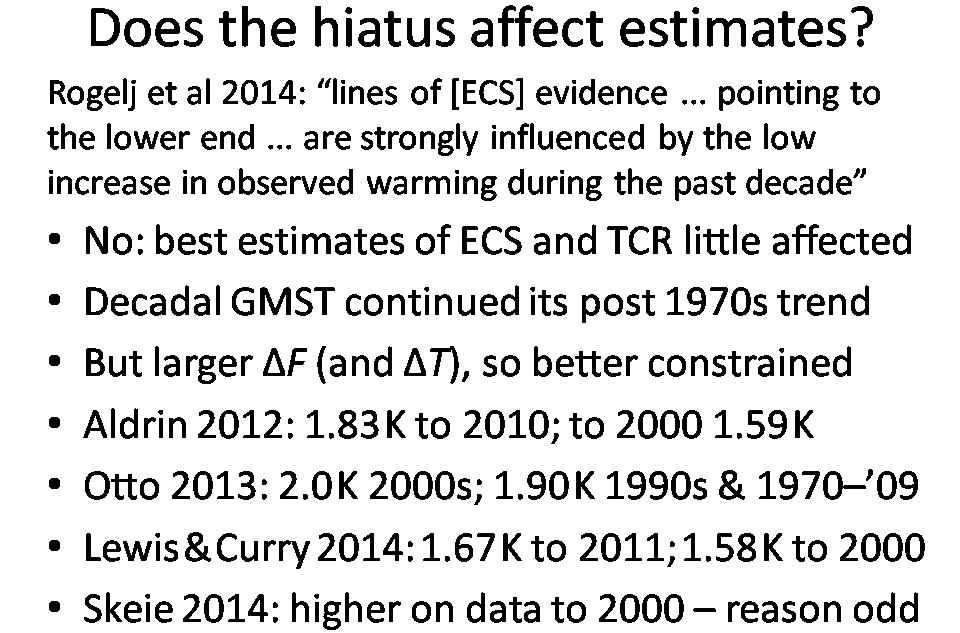
I’ll start with an easy target: claims that reduced instrumental period warming based ECS estimates that have been published over the last few years reflected the hiatus in warming over the last decade. Such claims are demonstrably false. The main effect of using data extending past 2000 is to provide better constrained ECS estimates, as the anthropogenic signal rose further above background noise.
Most recent studies that give results using data for different periods actually show lower, not higher, ECS median estimates when data extending only to circa 2000 is used. Skeie 2014 is an exception. I attribute this to the less strong observational constraints available from such data being unable to counteract its excessively negative aerosol forcing prior distribution.
Slide 20
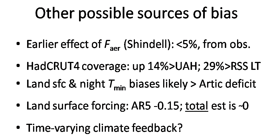
Now for some genuine issues. First, in a 2014 paper Drew Shindell argued that inhomogeneous forcing, principally by aerosols, with a greater concentration in the northern hemisphere – particularly in the extratropics – than homogenous GHG forcing would have a greater effect on transient global warming. That is principally because the northern hemisphere has more land and warms more rapidly. That aerosol forcing reached a peak level some time ago, unlike for GHGs, also contributes to the effect. The result would be that TCR, and hence ECS, estimates based on observed global warming were biased down.
I think there is in principle something in Shindell’s argument, but I regard his GCM-based estimate of the magnitude of the bias as absurdly high. Based on a simple model and observational constraints as to the ratios of transient warming for various latitude zones, I obtain a best estimate for the bias of no more than about 5%. It would be difficult to reconcile a significant bias with estimates from the non-energy budget ‘good’ studies being in line with energy-budget based estimates. Good non energy-budget studies should be unaffected by this issue due to their use of models that resolve forcing and temperature by hemisphere, and within each hemisphere by latitude zone and/or land vs ocean.
In his Ringberg talk, Gavin Schmidt stated that in the GISS-E2-R AOGCM, the transient responses (over ten years) to aerosol forcing and land use were respectively 1.33x and 3.65x as large as that to GHG forcing. From this he deduced that TCR and ECS estimated from the model’s historical run were biased low by about 20% and 30% respectively. Picking (over high) median estimates based on historical period unadjusted forcing, of 1.6°C for TCR and 1.9°C for ECS, he claims that these go up by respectively 35% and 60% when adjusted for forcing-specific ‘transient efficacy’.
I am at a loss to understand how the diagnosed increases of 20% and 30% turned into claimed increases of 37% and 63% – maybe this was achieved by using uniform priors. Moreover, the very large estimated land use forcing transient efficacy shown in Gavin Schmidt’s slide is based on an unphysical regression line that implies a very large GMST increase with zero land use forcing. In view of these oddities the findings shown seem questionable.
If, despite my doubts, the results Gavin Schmidt presented are correct for the GISS-E2-R model, they would support Drew Shindell’s argument in relation to that model. But it would not follow that similar biases arise in other models or in the real world. I am aware of only two other AOGCMs for which transient efficacies have been likewise been diagnosed using single-forcing simulations (Shindell 2014 used the standard CMIP5 simulations, which is much less satisfactory). One of those models shows a significantly lower transient efficacy for aerosol forcing than for GHG (Ocko et al 2014), behaviour that implies TCR and ECS estimates based on historical warming would be biased up, not down. The other model also appears to show that behaviour, albeit based only on preliminary analysis.
In the light of the available evidence, I think it very doubtful that aerosol and land use forcing have caused a significant downwards bias in observationally-based estimation of TCR or ECS.
The next two bullet points in slide 20 concern arguments that the widely-used HadCRUT4 surface temperature dataset understates the historical rise in GMST. However, over the satellite era, which provide lower troposphere temperature estimates with virtually complete coverage, HadCRUT4 shows a larger global mean increase than does UAH and, even more so, RSS. It seems quite likely that upward biases arising from land surface changes (UHI, etc.) and the destabilisation of the nocturnal boundary layer (McNider et al 2012) exceed any downwards bias resulting from a deficit of coverage in the Arctic.
For land surface changes, AR5 gives a negative best estimate for albedo forcing but states that overall forcing is as likely positive as negative. On that basis it is inappropriate to include negative land surface forcing values when estimating TCR and ECS from historical warming. Those studies (probably the majority) which include that forcing will therefore tend to slightly overestimate TCR and ECS.
The final point in this slide concerns the argument, put quite strongly at Ringberg (e.g., see here) that climate feedback strength declines over time, so that ECS – equilibrium climate sensitivity – exceeds the effective climate sensitivity approximation to it estimated from changes in GMST, forcing and radiative imbalance (or its counterpart, ocean etc. heat uptake) over the instrumental period. As explained in Part 1, in many but not all CMIP5 models global climate feedback strength declines over time, usually starting about 20-30 years after the (GHG) forcing is imposed. I address this issue in the next slide.
Slide 21

As running AOGCMs to equilibrium takes so long, their ECS values are generally diagnosed by regressing their top of atmosphere (TOA) radiative imbalance N – the planetary heat absorption rate – on dT, their rise in GMST, during a period of, typically, 150 years following a simulated abrupt quadrupling in CO2 concentration. The regression line in such a ‘Gregory plot’ is extrapolated to N = 0, indicating an equilibrium state. ECS is given by half the dT value at the N = 0 intercept. That is because CO2 forcing increases logarithmically with concentration, and a quadrupling equates to two doublings.
Slide 21, not included in my Ringberg talk, illustrates the potential bias in estimating ECS from observed warming over the instrumental period. It is a Gregory plot for the MPI-ESM-LR model (chosen in honour of the Ringberg hosts). The grey open circles show annual mean data, that closest to the top LH corner being for year 1. The magenta blobs and line show pentadal mean data, which I have used to derive linear fits (using ordinary least squares regression). The curvature in the magenta line (a reduction in slope after about year 30) indicates that climate feedback strength (given by the slope of the line) is decreasing over time.
CMIP5 model ECS values given in AR5 were based on regressions over all 150 years of data available, as for the blue line in the slide. I have compared ECS values estimated by regressing over years 21-150 (orange line), as in Andrews et al (2014), with ECS values estimated from the first 35 years (green line). Since the growth in forcing to date approximates to a 70-year linear ramp, and at the end of a ramp the average period since each year’s increase in forcing is half the ramp period, 35 years from an abrupt forcing increase is fairly representative of the observable data. As can be seen, the ECS estimate implied by the orange years 21-150 regression line is higher than that implied by the blue year 1-150 regression line, which in turn exceeds that implied by the green years 1-35 regression line. This indicates an increase over time in effective climate sensitivity.
On average, ECS diagnosed for CMIP5 models by regressing over years 21-150 of their abrupt 4x CO2 Gregory plots exceeds that diagnosed from years 1-35 data by 19%. However, excluding models with a year 21-150 based ECS exceeding 4°C reduces the difference to 12%. This is fairly minor. The difference is not nearly large enough to reconcile the best estimates of ECS from observed warming over the instrumental period with most CMIP5 model ECS values. And it is not relevant to differences between observationally-based TCR estimates and generally higher AOGCM TCR values.
It is, moreover, unclear that higher AOGCM ECS values diagnosed by Gregory plot regression over years 21-150 are more realistic than those starting from year one. Andrews et al (2014) showed, by running the HadGEM2-ES abrupt 4x CO2 simulation for 1290 years (to fairly near equilibrium), that the ECS diagnosed for it from regressing over years 21-150 appears to be substantially excessive. The true model ECS appears to be closer to the estimate based on regressing over years 1-35, which is 27% lower.
Importantly, an increase in effective climate sensitivity over time, if it exists, is almost entirely irrelevant when considering warming from now until the final decades of this century. The extent of such warming, for a given increase in GHG levels, is closely dependent on TCR, irrespective of ECS. Even if effective climate sensitivity does increase over time, that would not bias estimation of TCR from observed historical warming. And the projected effect on warming from effective climate sensitivity increasing in line with a typical CMIP5 model would be small even over 300 years – only about 5% for a ramp increase in forcing, if one excludes HadGEM2-ES and the Australian models (two of which are closely related to it, with the third being an outlier).
Slide 22
Although the increase in effective climate sensitivity, due to a reduction in climate feedback strength, with time in many CMIP5 models appears to have little practical importance, at least on a timescale of up to a few centuries, finding out why it occurs is relevant to gaining a better scientific understanding of the climate system.
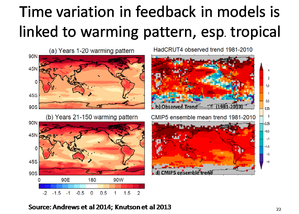
In a model-based study, Andrews et al (2014) linked the time-variation to changing patterns of sea-surface temperature (SST), principally involving the tropical Pacific. In current AOGCMs, after an initial delay of a few years, on a multidecadal timescale the eastern tropical Pacific warms significantly more than the western part and the tropical warming pattern becomes more El-Nino like, affecting cloud feedback.
The two LH panels in slide 22, from Tim Andrews’ paper and talk, show the CMIP5 model ensemble mean patterns of surface warming during the first 20 and the subsequent 130 years after an abrupt quadrupling of CO2. The colours show the rate of local increase relative to that in GMST. It can be seen that even during the first 20 years, warming is strongly enhanced across the equatorial Pacific.
The RH panels, taken from a different paper, show observed and modelled patterns of warming over 1981–2010. The CMIP5 ensemble mean trend (bottom RH panel) shows a pattern in the tropical Pacific fairly consistent with that over the first 20 years of the abrupt 4x CO2 experiment, as one might expect. But the observed trend pattern (top RH panel) is very different, with cooling over most of the eastern tropical Pacific, including the equatorial part.
So observations to date do not appear consistent with the mean evolution of eastern tropical Pacific SST predicted by CMIP5 models. Given Tim Andrew’s finding that weakening of climate feedback strength over time in CMIP5 models is strongly linked to evolving eastern tropical Pacific SST patterns, that must cast considerable doubt on whether effective climate sensitivity increases over time in the real world.
Slide 23
There are other reasons for doubting the realism of the changing SST patterns in CMIP5 models that Andrews et al (2014) found to be linked to increasing climate sensitivity.
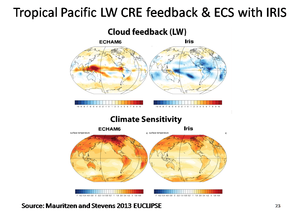
The strong warming in the deep tropics across the Pacific over years 21–150 is linked to positive longwave (LW) cloud feedback, which in CMIP5 models strengthens and spreads further after years 1–20. But is this behaviour realistic? In parallel with MPI’s main new CMIP6 model MPI-ESM2 (ECHAM6 plus an ocean module), Thorsten Mauritzen has been developing a variant with a LW iris, an effect posited by Dick Lindzen some years ago (Lindzen et al 2001). The slides for Thorsten Mauritzen’s Ringberg talk, which explained the Iris variant and compared it with the main model, are not available, but slide 23 comes from a previous talk he gave about this work. It shows the equilibrium position; so far only simulations by the fast-equilibrating slab-ocean version of the Iris model have been run. [Note: the related paper, Mauritsen and Stevens 2015, has now been published.]
As the top panels show, unlike the main ECHAM6/MPI-ESM2 model, the Iris version exhibits no positive LW cloud feedback in the deep tropical Pacific. And the bottom panels show that, accordingly, warming in the central and eastern tropical Pacific remains modest. This suggests that, if the Iris effect is real, any increase in effective climate sensitivity over time would likely be much lower than CMIP5 model ensemble mean behaviour implies. The Iris version also has a lower ECS than the main model, although not as low as might be expected from the difference in LW cloud feedback, as this is partially offset by a more positive SW cloud feedback.
Slide 24
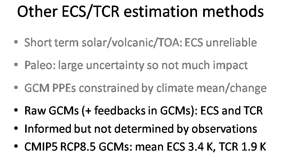
Slide 24 lists methods of estimating ECS other than those based on observed multidecadal warming. I explained in Part 1 that I concurred with AR5’s conclusions that estimating ECS from short term responses involving solar or volcanic forcing or TOA radiation changes was unreliable, and that true uncertainty in paleoclimate estimates was larger than for instrumental period warming based estimates. That implies that combining paleo ECS estimates with those based on instrumental period warming would not change the latter very much.
I also showed, in Part 2, that the model most widely used for Perturbed Physics/Parameter Ensemble studies, HadCM3/SM3, could not successfully be constrained by observations of mean climate and/or climate change, and so was unsuitable for use in estimating ECS or TCR. (Such use nevertheless underlies UKCP09, the official UK 21st century climate change projections.)
The other main source of ECS estimates involves GCMs more directly. Distributions for ECS and TCR can be derived from estimated model ECS and actual model TCR values. A 5-95% ECS range for CMIP5 models, of 2–4.5°C, was given in Figure 1, Box 12.2 of AR5. Feedbacks exhibited by GCMs can also be analysed, and to some extent compared with observations. But although development of GCMs is informed by observations, their characteristics are not determined by observational constraints. If the climate system were thoroughly understood and AOGCMs accurately modelled its physical processes on all scales that mattered, one would expect all aspects of their behaviour to be fairly similar, and the ECS and TCR values they exhibited might then be regarded as reliable estimates. However, those requirements are far from being satisified.
Since AOGCMs tend to be similar in many respects, it is moreover highly doubtful that a statistically-valid uncertainty range for ECS or TCR can be derived from CMIP5 model ECS and TCR values. If some key aspect of climate system behaviour is misrepresented in (or unrepresented by) one CMIP5 model, the same problem is likely to be common to many if not all CMIP5 models.
In this connection, I’ll finish by highlighting two areas relevant to climate sensitivity where model behaviour seems unsatisfactory across almost all CMIP5 models.
Slide 25
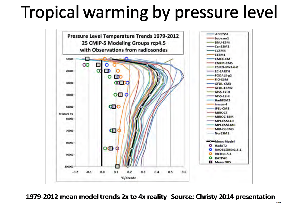
Slide 25 compares tropical warming by pressure level (altitude) in CMIP5 models and radiosonde observations over 1979-2012. Most models not only show excessive near-surface warming, by a factor of about two on average, but a much greater increase with height than observations indicate. This is the ‘missing hot-spot’ problem. The ratio of tropical mid-troposphere to surface warming would be expected to be smaller in a model with a LW iris than in one that does not, a point in favour of such a feature.
Figure 9.9 in AR5 showed much the same discrepancy – an average factor of about 3x – between observed and modelled temperature trends in the tropical lower troposphere over 1988-2012. Observations in that case were based on satellite MSU datasets and reanalyses that used models to assimilate data.
Slide 26

A lot of the discussion at Ringberg 2015 concerned clouds, one of the most important and least well understood elements of the climate system. Their behaviour significantly affects climate sensitivity.
Slice 26 shows errors in cloud fraction by latitude for twelve CMIP5 GCMs. (TCF)sat. is the average per MODIS and ISCCP2 observations. It can be seen that most models have too little cloud cover in the tropics and, particularly southern, mid latitudes, and too much at high latitudes. Errors of this magnitude indicate that reliance should not be placed on cloud feedbacks exhibited by current climate models.
Models also appear to have excessive low cloud liquid water path, optical depth and albedo, which may result in negative optical depth climate feedback being greatly underestimated in models (Stephens 2010).
Slide 27

My concluding slide reiterates some of the main points in my talk. Assuming Bjorn Stevens’ revised estimate of aerosol forcing is correct, then the 95% uncertainty bounds on ECS and TCR from observed multidecadal warming are well below the mean ECS and TCR values of CMIP5 models. It will be very interesting to see how these discrepancies between models and observations are resolved, as I think is likely to occur within the next decade.
Additional references
Timothy Andrews, Jonathan M. Gregory, and Mark J. Webb (2015): The Dependence of Radiative Forcing and Feedback on Evolving Patterns of Surface Temperature Change in Climate Models. J. Climate, 28, 1630–1648
Lindzen, RS, M-D Chou, AY Hou (2001) Does the Earth have an adaptive infrared iris? Bull. Amer. Meteor. Soc. 82, 417-432, 2001
Mauritsen, T and B Stevens (2015) Missing iris effect as a possible cause of muted hydrological change and high climate sensitivity in models. Nature Geoscience doi:10.1038/ngeo2414
McNider, R. T., et al. (2012) Response and sensitivity of the nocturnal boundary layer over land to added longwave radiative forcing. J. Geophys. Res., 117, D14106.
Ocko IB, V Ramaswamy and Y Ming (2014) Contrasting Climate Responses to the Scattering and Absorbing Features of Anthropogenic Aerosol Forcings J. Climate, 27, 5329–5345
Rogelj J, Meinshausen M, Sedlácek J, Knutti R (2014) Implications of potentially lower climate sensitivity on climate projections and policy. Environ Res Lett 9. doi:10.1088/1748-9326/9/3/031003
Shindell, DT (2014) Inhomogeneous forcing and transient climate sensitivity. Nature Clim Chg: DOI: 10.1038/NCLIMATE2136
Stephens, GL (2010) Is there a missing low cloud feedback in current climate models? GEWEX News, 20, 1, 5-7.
Update 21 April 2015
The Mauritsen and Stevens paper about the new MPI Iris model has just been published. I have added a reference to it, and to a couple of inadvertently omitted references.


98 Comments
Thank you Nic. This is one of the big picture posts that helps me to hang together many of the ideas I have learned over the last 7-8 years. This presentation (of your Ringberg presentation) is a goldmine of clear ideas and methodological thinking. I look forward to several readings. I am indebted to you.
Thanks for your kind comment, Mark
“The strong warming in the deep tropics across the Pacific over years 21–150 is linked to positive longwave (LW) cloud feedback, which in CMIP5 models strengthens and spreads further after years 1–20. But is this behavior realistic? ”
“Models also appear to have excessive low cloud liquid water path, optical depth and albedo, which may result in negative optical depth climate feedback being greatly underestimated in models (Stephens 2010).”
Judith Curry’s comment today at CE: “From what I understand, cloud feedbacks are negative – a stabilizing effect on climate whether it is warming or cooling.”
Nic, in your Part II when I asked if ECS/TCR could vary over temperature you replied: “I’m not aware of much evidence that TCR or ECS is materially temperature dependent, within a span from a degree or two colder than now up to four or five degrees warmer, although this is based mainly on model simulations.” But now you are saying that the models are getting both cloud development patterns and cloud feedback wrong. And Dr. Curry is saying that cloud feedback is temperature or climate dependent, “a stabilizing effect.” Wouldn’t these statements show belief evidence that TCR is temperature or climate dependent?
Ron,
Climate feedbacks by definition are effects on readitive imbalance that vary with temperature. But only if they are nonlinear in temperature – so that the feedback strength varies with the climate (average temperature) state – would it imply that TCR or ECS were climate state/ mean temperature dependent.
I should have qualified that it’s given that GMST is a function of ECS/TCR in a linear relationship. But considering a major portion of that relationship is vapor and cloud feedback, and considering both of these could have non-linear and possibly independent relationships to temperature, would it not be highly plausible that ECS/TCR is also non-linear to GMST? For example, when the tropics reach a threshold there is increased cloud cover but also increased precipitation, so cloud albedo increases but humidity no so much. Could this impose an increasing climate resistance if cloudiness tracked Clausius Clapeyron?
Want to ask about Dessler’s Ringberg presentation. He has a few interesting things to derive ECS from CERES and MERRA data. He gets to ECS of 3.5C but a lot of it is due to positive cloud feedback!
He is using the radiative kernels and Held and Shell decomposition of feedbacks (I believe this reference http://citeseerx.ist.psu.edu/viewdoc/download?doi=10.1.1.221.3936&rep=rep1&type=pdf), that uses RH – relative humidity – as a parameter. This breaks out the feedbacks differently from the traditional list used by IPCC etc.
Assuming RH is approx constant, he gets a lambda-total fixed-cloud, based on feedbacks of -1.87+/-.20 W/m2/K translating to ECS of 1.8-2.2C. But then clouds add to it by 0.87 to give -1.07 lambda to produce ECS of 3.5C.
Dessler states: “Cloud feedback very likely positive; estimate of 0.8 W/m2/K” Hmmm. Original IPCC formulation has much of the positive feedback in the ‘water vapor’ category. Is the Held and Shell moving definitions around? And if not, how can he argue for large positive cloud feedback, given his own 2008 paper which has a fairly weak signal (0.1 W/m2/K I think) or Spencer Braswell showing negative? He cites “Chen Zhou et al in prep.” on this.
So his conclusion is ECS of 3.5C, but the derivation made leaves the open question – If cloud feedback is negative or non-positive, is the implication that ECS would be 2.0C? If so, how come traditional IPCC feedbacks have higher ECS with not so large cloud feedback?
Suggestion to McIntyre: Maybe a “Ringberg roundup” to analyze the Ringberg presentations? Deconstructing these talks would be informative for us layman observers. This and other Ringberg presentations raise interesting questions.
patmcguiness,
Good questions. I need to study Dessler’s slides properly. At this point I don’t know whether what he has done makes sense or not. My understanding is that it is very difficult to draw conclusions about global feedback strength from short term variations in TOA radiation. And the correlation in Dessler’s first plot is evidently very small.
The Held and Shell decomposition struck me as quite sensible when I read about it, but I have no experience with it, so I can’t answer your question.
You might like to read Dessler’s 2013 J Climate paper that he cites in his talk, available here: http://geotest.tamu.edu/userfiles/216/dessler2013.pdf , and leave a further comment with any thoughts you have on it.
You say: If so, how come traditional IPCC feedbacks have higher ECS with not so large cloud feedback?
This may be because in most (not all) CMIP5 models, climate feedback strength deceases over time, so that ECS exceeds what it would be if calculated based on shortish-term (even multidecadal) feedbacks.
Comments in light of reading Dessler 2013 right now.
“My understanding is that it is very difficult to draw conclusions about global feedback strength from short term variations in TOA radiation. And the correlation in Dessler’s first plot is evidently very small.”
Probably so, but in Dessler’s defense, he note the only data that’s good is about 10 years worth of TOA and other high quality data, so doing short term feedbacks is the best you can do. Looking under the lamppost problem. Spencer, Lindzen, and many others) have done the same; they’ve had arguments with Dessler mainly about lead and lag times and interpretation, and Dessler did some suspect work in discounting data that showed lower relative humidity (Partridge) on the basis of short-term feedback data used to make a long-term point.
Table 1 has feedback breakdown. And it does seem that the constant RH-based feedback re-allocates the water vapor, lapse rate and planck feedbacks, but doesnt change the definition of cloud feedback. Which sort of answers my question. I dont quite understand how Dessler 2008 had
Longwave and shortwave cloud feedback on temp both positive is counterintuitive, given the net large -20W/m2 negative feedback in clouds. Doubts only grow looking at Fig 1 scatter plot. It’s a mess. Albedo feedback is a much cleaner and desirable (flattish) trend, but cloud is a shotgun blast plot. This similar btw to a prior Dessler paper that was a ‘rebuttal’ to Spencer – scatter shot to show (slight) positive feedback. I look at the other three (temp, albedo, water vapor) and it gives confidence in the linear regression, but the cloud doesnt. His numbers on ERA was 0.49 W/K and MERRA 0.58 W/K. Still below the 0.81 W/K.
Dessler: “The total cloud feedback in the observations shows negative cloud feedbacks in the deep tropics (158S–68N)and high southern latitudes (408–758S) and positive cloud feedbacks at most other latitudes. Averaging over the globe yields a positive total cloud feedback. As this plot makes clear, attempts to determine the cloud feedback by looking just at a particular latitude range, such as 208N–208S (e.g., Lindzen and Choi 2009) are likely to be considerably in error. Compared to observations, the control ensemble
overestimates the positive longwave cloud feedback in the tropics and underestimates the negative shortwave
cloud feedback there. These errors add, and the control ensemble ends up with a positive total cloud feedback in the tropics, opposite to that seen in the observations.”
Now Dessler disses Lindzen and Choi by saying they are just covering the tropics, but most of the power of feedback is in those areas. Lindzen and Choi said: “… the water vapor feedback is almost certainly restricted primarily to the tropics, and there are reasons to suppose that this is also the case for cloud feedbacks.”
The lack of tropical ‘hot spot’ and cloud feedback error in the tropics is perhaps related; it’s been a mystery that impacts both water vapor feedback and clouds. Dessler goes on to say that errors in tropics and other latitudes balance out to get approximately correct average, so its all good. Dessler seems to be attributing correlations to causation/feedback, and one could envision alternative explanations (such as what Spencer & Braswell did). Using short-term feedback data to develop long-term feedbacks is another concern.
As an informed layman, I dont have the depth of understanding to know the right answer to various claims and counterpoints; They are teasing out signals from noise in ways that are highly subject to interpretation. While parts of the signal seems clear, the cloud feedback continues to be an area where signal to noise seems low.
Dessler, like so many in climatology, seems blissfully unaware of valid use of OLS and the consequences of not respecting the necessary condition of minimal x-axis error.
In short regression dilution. Significant x error will reduce the slope estimation. In rad vs temp, that means it exaggerates climate sensitivity. This was mentioned in Forster & Gregory 2006, so one wonders whether this is really so unknown in the field.
I wrote about this in detail here:
In the case of Dessler 2013 figure 1 (top-right) it blatantly obvious to the naked eye that the slope grossly underestimated by his OLS fit. The suggested 95% confidence range is meaningless since it does not take account of this major cause of error in the slope.
Similarly top left is seen to be too low on inspection. The round blob of data in lower left plot is so uncorrelated as to make even suggesting a linear regression farcical.
Lower-right may not be too far off but will necessarily suffer from some bias. The plot is too poorly scales to tell by inspection.
Trenberth and many others repeat this error. It is endemic in climate science.
The only ones I have seen address the problem are: F&G ( though they avoid citing the problem in their conclusions and tuck the whole discussion away in an appendix ); and Lindzen.
The other huge problem with this whole approach is that it confounds the immediate response where a change in forcing produces at *rate of change of temperature* with the equilibrated response of a final temperature change.
This latter point is probably one reason why the slope reduces with time as Nic explains here. Another reason is that the Planck response is not, in fact, linear but T^4.
Greg Goodman.
Looks like Bjorn Stevens has a new paper in Nature Geoscience on missing Iris effect in climate models.
Was Gavin Schmidt’s new land use calculation based primarily on his irrigation/cooling effect analysis?
Regardless, if one accepts his position it seems to reduce the probability that natural variability is the culprit behind continued GCM (or at least GISS-E2-R) failures.
That is unclear to me, but it seems quite possible.
“The next two bullet points in slide 20 concern arguments that the widely-used HadCRUT4 surface temperature dataset understates the historical rise in GMST. However, over the satellite era, which provide lower troposphere temperature estimates with virtually complete coverage, HadCRUT4 shows a larger global mean increase than does UAH and, even more so, RSS. It seems quite likely that upward biases arising from land surface changes (UHI, etc.) and the destabilisation of the nocturnal boundary layer (McNider et al 2012) exceed any downwards bias resulting from a deficit of coverage in the Arctic.”
Nick,
I’m traveling so I may not have time for a back and forth but it is not ‘very likely’ that land surface changes and nocturnal boundary layer changes exceed biases from a deficit of coverage in the Arctic. That’s such a hand-waving argument which isn’t based on science. In fact, there is very little observational evidence that UHI provides any sort of of long-term trends when this issue has been examined in detail. Perhaps it would be worthwhile for you to chat with Mosher and Zeke a little about this…
Secondly,
Satellite temperature trends are interesting and useful products but they still have remaining issues and there is a large discrepancy between the results of the three major groups (UAH, RSS, STAR). There has even been studies published in the last two months by Chidley (I believe) which challenge one of the corrections used in the UAH (has a big effect on trends). Not to mention that RSS supposedly has a spurious cooling trend according to Spencer. All in all there are more reasons to be skeptical of the satellite products than the much more reliable and replicated surface record. One of the key points about Arctic warming is that its vertical structure is strongly concentrated in the near-surface over the past two decades therefore satellite lower atmosphere trends will underestimate the nature of these changes in the Arctic.
Overall, there is a far greater likelihood that satellite datasets are biased low as opposed to the surface temperature network.
I find Nic’s arguments for clinging to Hadcrut unpersuasive. It would be far more convincing to actually do the estimate using the various data products ( had, C&W, giss, BE) and actually see what kind of difference we are debating rather than appealing to the UHI argument and satellite data argument.
On UHI for example Hadcrut has higher percentage of urban stations because of their reliance on long records which tend to be in urban settings.
Steven,
It is very simple to work out what difference using the Cowtan & Way or the sea-ice-from-air-temperature version of BEST rather than HadCRUT4 makes to ECS and TCR estimates based on multidecadal global warming. They scale pro rata to the increase in GMST used. For the main long period used in Lewis & Curry 2014, 1859-82 to 1995-2011, the difference is about 8%. For the shorter period used, 1930-50 to 1995-2011, it is about 3%. for Lewis (2013) J Clim, which reached an almost identical best estimate for ECS to Lewis & Curry (2014) and supports a lower TCR estimate than that study does, non-global observational coverage for surface temperature is irrelevant since the model simulation output is masked to match the available observations.
I am not presently convinced that infilling large areas where there is little or no reliable nearby data is sensible. I certainly regard GISS’s extrapolation approach as unsatisfactory, and the use by both GISS and C&W of the stitched together Bromwich reconstruction for Byrd in Antarctica as being unsupportable.
Nic
‘I am not presently convinced that infilling large areas where there is little or no reliable nearby data is sensible. ”
you are ALWAYS infilling. CRU infills.
In short the CRU estimate of the globe (with missing data ) is no different than the same estimate with the missing data replaced by the global average. That is, the global average of CRU is a tactic infilling of the missing data with the global average.
This approach will necessarily bias your estimate if the missing data is located in an area where there is more warming or more cooling than average.
For example, if all my missing data were from rural areas people would suely complain that are average had the potential for a warming bias.
The arctic is warming more than the rest of the planet. Infilling it (tacticly ) as CRU does with the global average trend biases the global average downward.
We can tell that CRU is biased low by looking at out of sample data
1. The stations that they leave out because they cant use short records
2. Reanalysis, which is a physics based infilling
3. Artic bouys, which CRU cant use
4. Comparison with satellite products that measure the surface ( AIRS )
You can also look at how trends in temperature change as a function of latitude.
Up to 80N we see an increasing trend as a function of latitude. When CRU avoid infilling, they are tacitly asserting that the area north of 80 has the same trend as the planet as a whole. In other words they assert that the trend north of 80 is less than the trend at say 75N. Giss assert that te trend north of 80 is the same as the trend at 80. C&W use ALL the information to make a more informed prediction and then they actually TEST that prediction with different data sources.
Finally in a synthetic test of the three methods ( RSM, CAM and Kriging ) I’m sorry but Krigging wins.
Re Mosher:
“”That is, the global average of CRU is a tactic infilling of the missing data with the global average.””
1. They really use global average????
“”This approach will necessarily bias your estimate if the missing data is located in an area where there is more warming or more cooling than average.””
“”For example, if all my missing data were from rural areas people would suely complain that are average had the potential for a warming bias.””
“”The arctic is warming more than the rest of the planet. Infilling it (tacticly ) as CRU does with the global average trend biases the global average downward.””
2. The arctic is warming more than the rest of the planet?
How do you know this? From the infilled data? That statement has been made too many time with no proper documentation. It should be boiling by now.
What actual stations with a long history were used for this “warming”? How does it compare with the 1930’s and 1940’s?
3. What percentage of station data is being infilled now?
Is it 40 percent?
GM “The arctic is warming more than the rest of the planet?”
From Freeman Dyson, not a warmist: “The effect of carbon dioxide is important where the air is dry, and air is usually dry only where it is cold. Hot desert air may feel dry but often contains a lot of water vapor. The warming effect of carbon dioxide is strongest where air is cold and dry, mainly in the arctic rather than in the tropics, mainly in mountainous regions rather than in lowlands, mainly in winter rather than in summer, and mainly at night rather than in daytime. The warming is real, but it is mostly making cold places warmer rather than making hot places hotter. To represent this local warming by a global average is misleading.” See http://edge.org/conversation/heretical-thoughts-about-science-and-society
This doesn’t directly answer your question about data, but it does supply the explanation of a very accomplished scientist without a warmist axe to grind.
JD
Gerald Machnee –
They really use global average????
No, HadCRUT4 ignores areas with no temperature measurement. Mosher’s point — I think he intended “tacit” not “tactic” — is that mathematically, the HadCRUT average over measured areas gives the same result as a global average, in which the unmeasured areas have been assigned the average temperature of the measured areas.
RE JD Ohio
**This doesn’t directly answer your question about data, but it does supply the explanation of a very accomplished scientist without a warmist axe to grind.**
It is a theory but does not supply a measurement. Even if it worked, the effect of the CO2 would be very small, not the whole degrees that has been thrown around. Check the Eureka temperatures and see what they have done. Eureka has only been there since about 1950, but a few others have been there longer.
As Steven Mosher correctly points out, not explicitly infilling in the manner that HadCRUT does it, is equivalent to infilling with the global mean.
To respond to Geral Machnee’s comments, it is our expectation, confirmed with limited measurements as well as weather-model based reanalyses by e.g. ECMWF or NCEP, that there is a polar amplification of any warming (and cooling).
So I think we can with good confidence treat the warming observed by the HadCRUT index as a lower limit on the global warming of the Earth.
Certainly it must be possible to do “a better job” (provide a less biased method for infilling) than is done by HadCRUT.
My initial complaint with Robert Way’s work was the use of a simplistic hybrid satellite-surface temperature model. Regardless of what people say, satellite-based measurements do not attempt to measure the 1-m above surface air temperature in the atmospheric surface boundary layer. Rather they are an average over the lower tropospheric radiometric temperature. The physics is different so what you are measuring is different (short-period climate variability is seen with different amplitudes and latencies, etc).
Anyway, they’ve certainly improved their analysis more recently by the use of multiple methods for infilling. But when you look at the impact of that infilling, the results are relatively modest. [The units are °C/decade.]
It is an unfortunate tendency on their part to serially exaggerate the importance of the effect of the infilling by reporting the relative impact on the (nearly cancelled) global temperature trend on the 1997-(as then current):
As I’ve pointed out before, the trend from 1997-2013 is heavily influenced by regional scale variability and in principle could take either sign or even be (within measurement error) zero. If you look at my chart from 2002-2012, HadCRUT global has a trend of -0.044 °C/decade where as C&W-Hybrid is 0.031. That ratio is -0.7 which clearly is a meaningless number.
Looking at the difference between trends reveals a very modest effect of about 0.06°C/decade. The relative importance of this correction is inflated because the central value happens to be near zero of the uncorrected quantity.
If you go from 1979-2012 (so you’ve eliminated more of the influence of short-period variability), you find 0.168°C/decade for HadCrut verus ironically 0.181°C/decade for C&W-Kriging. That suggests about a 7% bias.
But extending the period to 1959-1972, the two indices flip: HadCrut gives 0.132°C/decade whereas HadCRUT-Kriging is 0.130°C. I think this is a clear demonstration that the net effect of more physically plausible infilling methods does not yield a global mean temperature that is biased high relative to the HadCRUT index.
I think it’s useful to look at the issues with the missing regions from the 1859–1882 period using by Lewis and Curry (2014), especially since they are comparing that value to 1995-2011. It seems to me this must produce a bias in their ECS estimate (but it’s not obvious to me which sign this bias should have).
Cowtan & Way 2014 I think would be a good approach to looking at that effect.
For Steven Mosher,
While I agree that of RSM, CAM and Kriging, kriging wins in a perfect world, the world is not perfect.
Simply, bad kriging can be last on the list.
You have to have a quality objective.
In ore resource work, you need a bankable document in many cases.
Keen eyes scrutinise the work before the cheque arrives.
The question re C&W is whether there is a bankable standard.
I think not. There are fewer avenues available in their type of work, compared to ore resource work, to validate or verify.
The same applies to BEST.
It is no consolation that BEST gives a good match to other estimations. All are supposed to start with the same raw data available. One should be surprised if they do not agree. That does not say whether all have bias, or do not have bias.
Compared to historical data here in Oz, we do see bias. Like the alleged warming being two to three times the historical record quantity.
O/T – Steven Mosher mentions –
“Finally in a synthetic test of the three methods ( RSM, CAM and Kriging ) I’m sorry but Kriging wins.”
I may be wrong in recall, but i remember “Kriging” use being discussed at CA as a possible usefull tool in “Climate Science”.
it seemed a “black art” with on the ground/real world results to me at the time, but i never had the time to look deeper.
any thoughts anybody ?
dfhunter
yes kriging was mentioned many times at climateaudit. if you look through the literature OUTSIDE that devoted to global series you will find folks using kriging to do temperature series.
in short some skeptics said “use known methods, none of this home grown stuff”
in short they said “get stats on on the problem”
did both of those. the answer comes out “warmer”
now folks like the untested homegrown stuff.
go figure.
Regarding polar amplification- nice theory but Antarctica is even drier than the Arctic, and record sea ice there does not support the theory. Where is the Antarctic warming?
Nice theory, though.
Robert,
You are incorrect in implying that I said it was ‘very likely’ that land surface changes and nocturnal boundary layer changes exceed biases from a deficit of coverage in the Arctic. I said, as you correctly quote earlier, that it was ‘quite likely’. I’m open to persuasion otherwise by Mosher and Zeke.
I don’t know why you claim that my view are not based on science; I cited a peer reviewed paper that presented a detailed case about nocturnal boundary layer changes affecting trends in surface minimum temperatures. And one reference for changes affecting land surface use impacting temperature trends is McKitrick (2013) Encompassing tests of socioeconomic signals in surface climate data.
The difference between HadCRUT4 and Cowtan & Way appears to have little to do with a deficit of coverage in the Arctic per se, but rather primarily to be due to differences in the treatment of sea ice. This can be seen by examining GMST changes in the two versions of the BEST dataset. The version that estimates surface temperatures where there is sea ice from land air temperatures, the approach used by Cowtan & Way, generally agrees closely with Cowtan & Way. The version of BEST that estimates surface temperatures where there is sea ice from sea surface temperatures generally agrees closely with HadCRUT4.
I concur that the vertical structure of the atmosphere in the Arctic leads to surface warming exceeding tropospheric warming, unlike in most of the world. However, the UAH 1979-2013 trend from 65N polewards is not that far short of the GISS trend for polewards of 64N, which is based on infilling.
Your claim that “there is a far greater likelihood that satellite datasets are biased low as opposed to the surface temperature network” [being biased high] seems unsupported by the evidence to me, assuming it relates to the globe.
Nic:
“And one reference for changes affecting land surface use impacting temperature trends is McKitrick (2013) Encompassing tests of socioeconomic signals in surface climate data.”
I’ll speak a little about McKitrick 2013. It really doesnt address the issue, 2010 paper is the one you wanted.
A) ross’s data is corrupt, basically he makes a bunch of errors in geo locating sites. I informed him of this, but he argued that it doesnt matter. He didnt provide test to substantiate this.
B) his regression is dimensionally meaningless. Temperature is regressed as a function of literacy for example. Eskimo’s better not learn to read.
I should probably finish the work I have going on re doing Ross’s analysis with the correct metadata. One problem is that the socioeconomic data he cites is not available at the links he provided. Another problem is you have time series at different frequencies. That said, the 2013 paper does present an interesting methodological framework, I should probably finish the work I started down that path.
With regards to boundary layer issues I’ll have to dig into that one. I would place little confidence on findings I haven’t checked myself down to the bits.
regardless, IF UHI and boundary layer are a problem, they are a problem for ALL series and so the selection of CRU cannot be justified by appealing to these issues.
As for determinig whether or not satellite data is biased low we have a fundamental problem of data sharing and code sharing. Nobody in that field comes close to releasing the kind of data and code that you do. When poorly documented results are at odds with fully documented results, my sense is not to put a lot of faith in the poorly documented stuff.
Robert casts envious glances toward the quiet sky as he screams over the noisiness of his own data roar.
====================
Re Carrick:
**To respond to Geral Machnee’s comments, it is our expectation, confirmed with limited measurements as well as weather-model based reanalyses by e.g. ECMWF or NCEP, that there is a polar amplification of any warming (and cooling).**
I believe that the Weather-model based reanalyses of amplification is overused with not enough measurements to substantiate it.
Reflections from a clouded iris.
================
Nic, thanks for the link to the brand new Mautizen/Stevens paper. From the free supps: The iris-effect reduces the ECS of the used model (ECHAM6)from 2.81 to 2.21 (22%). This could be indeed a giant step for mankind (h/t N.Armstong) to come to more realistic climate models. And some of the “specialists” would have to offer an appologise to Lindzen…
Nic Lewis:
I think this is a mathematical physics issue, rather than one you can strictly argue from strictly empirical observations. So unfortunately, I do think the broader point is correct, regardless of whether Gavin Schmidt did his statistical analysis correctly.
Speaking just from the perspective of mathematical physics, if you have a system that has modes that have long latencies (such as the roughly 2000-year deep ocean coupling), you will need to observe the system for a sufficiently long period for these modes to kick in..
I would argue this is a fundamental limitation of trying to use a limited data set: That the absence of long latency responses to the system in your short period of observation is biasing your estimates of ECS is simply not something you can disprove by looking at ~150 year length data sets alone (you’d need a robust model to combine the measurements with in this case).
I would think even if there were much better agreement between the models and observation over the short time periods we have that we would still have no idea whether those models did a credible job ON much longer time SCALES, although I admit there would at least be an argument in the model’s favor in THAT CASE.
Carrick
I think you are conflating two issues here. Gavin Schmidt’s presentation was about short term, transient, responses to different forcing agents, not about effective climate sensitivity increasing over time.
I agree that a 150 year dataset (with most of the forcing increase taking place over the last 70 years) cannot in itself prove or disprove such behaviour. However, my arguments regarding the extent to which effective climate sensitivity may be biased low as an estimate of equilibrium climate sensitivity (ECS) relate to behaviour in AOGCMs.
If the the AOGCMs that exhibit increasing effective CS also exhibit a particular pattern of SST within a period of a few decades, the existing dataset may be long enough to support or disprove the existence of such a pattern in the real climate system. It is notable that in all the CMIP5 AOGCMs that exhibit an increase in effective CS over time, the slope of the Gregory plot alters fairly abruptly after about 20-30 years and then appears to be fairly linear until year 150, the point at which most of the abrupt 4x CO2 simulations were ended. To be certain of model behaviour beyond that point, longer simulations can be performed.
Carrick,
Seems to me that if you explicitly consider ocean heat uptake in the calculation of ECS by heat balance (a la Nic Lewis and others), then there is no need to be concerned about the instrumental data being limited to ~150 years.
Yes, the quality of data in the early part of the record adds some uncertainty to the calculated empirical estimate. Yes, substitution of Cowtan & Way high latitude estimates will increase the empirical sensitivity values modestly. Yes, there is the potential for ‘non-linearity’ of climate sensitivity with rising temperature (eg. Armour et al and others). But the empirical determination over the past 150 years at a minimum sets a defensible estimate which is relatively free of assumptions, and completely free of GCM influence. I understand that these estimates are considered by some to be prejudiced low. But IMO, the burden of proof that the true ECS value is in fact higher than the empirical estimates remains with those who claim it is in fact higher. I have seen absolutely nothing convincing of higher sensitivity…. only grotesquely kludged GCM projections.
I note here that the mean GCM projection of warming is comically wrong for the past 15 years. Do you think that the models really have enough credibility to discount directly calculated sensitivity estimates?
Steve, great comment but the first thing you taught me was try not to end with a rhetorical question. 😉
If I were cynical I would notice the following pattern: satellite temperature is direct, global and hard to bias but it’s lower GMST data trend is discounted because it’s lower precision than surface thermometer recording. The most precise surface recording is in the last 20 years but it’s lower GMST data trend is discounted because of the anomaly said to be interfering with the CAGW signal. The use of direct observation with the the full 150-year surface shows a lower ECS but it is discounted because the beginning years were too uncertain and 150 years is not long enough a data set. All are replaced with models that were tested (“validated”) against the 150-year uncertain record but which failed their first predictive test which was the GMST would not significantly deviate from it’s diagnosed recent trend. Nic, thanks for your work and conviction, and toleration of my silly questions.
Steve, I will check out Armour.
Nic Lewis—I haven’t read Gavin’s RIngberg talk yet, so I definitely ended up conflating issues.
If I remember correctly, they typically run for longer than 150 years though to estimate ECS in the models…. Isaac Held describes a method where they run for 600 years for example.
Steve Fitzpatrick—I don’t think this helps. It’s a measurability issue. If you had a noiseless system with zero measurement error (and you knew the pole-zero structure), you could practically extrapolate the system response from a much shorter period than the actual response time of the system.
In practice, the system is not noiseless, the measurements are not noiseless, and not only do we not know the pole-zero structure, that structure is likely evolving over time.
This isn’t actually related to my criticism, which isn’t related to what GCMs say, but the physical constraints on the measurements from e.g. the thermal mass associated with the deep ocean.
But in my opinion, 15 years is way to short of a period for testing climate models versus data to the point of being utterly meaningless. I think you need at least 30-years of data, and that’s only if there isn’t a true 60-year AMO. If the AMO oscillation is real, you’ll need to be able to model the effects of that AMO on your measurements before you can reliably estimate ECS. Even 150 years of data is marginal in that case.
Carrick
The CMIP5 abrupt 4x CO2 simulations required a 150 year run; only for two GFDL-ESM2 models are longer (300 yr) runs archived. Those GFDL models seem to have much longer ocean timescales than any other CMIP5 models. The model ECS values given in AR5 Table 9.5 come from Forster et al 2013 JGR, and were derived from Gregory plot regression lines over years 1-150. They are probably low for the two GFDL models, but for HadGEM2-ES, a model with strongly non-linear feedback strength for which a very long 4x CO2 simulation was performed, the yrs 1-150 regression line seems to give an accurate estimate of actual model ECS.
I entirely agree that 15 years is too short to compare model and real world warming, although the model ensemble 15-year trend is a reasonable measure of how fast underlying model-average warming is.
NIc:
Im curious about you opinion of the very concept of the multi model ensemble mean…
are the multiple runs of various models independent from each other?
are multiple runs of the same model independent from themselves?
What exactly should one infer from a multimodal mean?
BTW: not meant as rhetorical questions at all.
Thanks, david
davideisenstadt,
I’m pretty dubious about the concept of a multimodel ensemble mean. The models are not independent of each other, and most or all of them appear to be too sensitive. And it is fairly arbitrary which models go to make up the mean – there was no quality test for CMIP3 or CMIP5, and multiple variants of the same model may be included. And sometimes each run is included despite the fact that some model may have ten runs and others only a single run, whilst other times the models are given equal weights. But the mean is used for all sort of purposes, both in climate science and for policy.
Multiple runs of the same model seem to be fairly independent of each other as regards sampling different realisations of internal model variability goes, but they obviously all reflect the underlying model properties, including ECS, TCR, etc.
All I would infer from the multimodel mean is how the set of models involved behave on average.
Nic Lewis, when they aren’t doing something similar to what Isaac Held does, and in particular only using a 150-year period, I believe we can legitimately question the reliability of their estimates of the model ECS.
It’d be interesting to compare for model runs like Held, the estimates from 150-years against the estimate from the full 600-year period.
Regarding intermodel comparisons, if you selected only models with similar resolution and physics, then combing the runs from each model is roughly the same as combining multiple runs from one model. What you’d be primarily learning about from that ensemble is internal variability of the model’s climate
The fact the ECSs vary so widely between relatively similar models is a smoking gun that the models aren’t inter-comparable in that way. In that case, I don’t have any idea what the mean of that ensemble is supposed to be giving you. As James Annan points out, this ensemble certainly isn’t truth centered.
Carrick,
The GFDL-ESM2G/M models seem pretty much unique in their very slow response. I believe GFDL estimates their ECS values both to be ~3.2 K. I don’t know what a regression estimate over the full 600 year abrupt 4x CO2 simulation is.
Over the first 150 years, the ECS regression estimate is 2.35 K for ESM2G and 2.45 K for ESM2M (to nearest 0.05 K). Regressing over years 21-150 increases the estimates to 2.8 K and 2.7 K respectively. Regressing over the full archived simulation, years 1-300, gives ECS estimates of 2.6 K and 2.7 K, whilst regressing over years 21-300 gives 2.85 K and 2.9 K. So for these models even 300 years is a bit too short. But, as I said, they seem to be exceptional in the great slowness of their reeponse.
davideisenstadt
As just a follow on from Nic’s response I happened to be looking at semi-empirical models for sea level rise and came across Bolin et al “Statistical prediction of global sea level from global temperature”, Statistica Sinica, that along the way needs to address this issue.
They say:
“It is worth noting that some modeling groups have more than one model in this selection [CMIP5]. Commonly such models have some code in common, and assuming that these models are independent or exchangeable, and that the union of them constitute an estimate of the between-model variability, is an oversimplification (Jun et al. (2008)). This variability is undoubtedly an underestimate, but it is not easy to correct for it. However, the spread in these temperature projections yields a better uncertainty quantification than the common approach to average all the projections.”
The reference to Jun et al is to “Spatial analysis to quantify numerical model bias and dependence: How many climate models are there?” J of the ASA 103. Its abstract concludes:
“Our results suggest that most of the climate model bias patterns are indeed correlated. In particular, climate models developed by the same institution have highly correlated biases. Also, somewhat surprisingly, we find evidence that the model skills for simulating the mean climate and simulating the warming trends are not strongly related.”
NIC and HAS:
thank you both for your responses.
Carrick, on reflection, I think I read that GFDL had found that their original 3.2 K ECS estimate for their ESM2G/M models was too high. It was based on the ECS of their similar CM2.1 model, but IIRC it turned out that the CM2.1 preindustrial control run had not fully equilibriated when they increased CO2 concentration to estamate ECS. So maybe the 300 year regression is long enough to give a fairly good ECS estimate for the ESM2G/M models.
Nic, a couple of questions.
1) If the rate of change in forcing is constant, would you expect that the temperature response would become constant as well?
2) If the apparent 60yr cycle in GMST is due to an underdamped oscillation in ocean response, would this have any impact on the calculation of ECS? i.e. Could it be that at the top of the cycle, that the SST is above equilibrium?
My guess is that the answer to Q1 is “approximately yes”. For Q2 I’m guessing “absolutely not”, but thought it an interesting question.
AJ, thanks for your questions:
1) Yes over periods of up to a few decades. As long as both climate feedback strength (variously alpha or lambda) and the ratio of ocean etc heat uptake to temperature change (kappa) are constant, the rate of GMST change dT/dt will be proportional to the rate of forcing change dF/dt. But as the ocean below the mixed layer warms up, it absorbs heat less readily, so kappa falls. One can see this effect operating in climate model simulations where the CO2 level increases by 1% p.a., giving a constant rate of increase in forcing. GMST gradually rises at a faster rate – dT/dt increases – although the effect is very small until six or seven decades have elapsed.
2) I don’t think that there is an y real significance in whether SST is at above equilibrium temperature at the top of a natural ~60 year cycle. That is by definition not an equilibrium state. What is important for estimation of ECS is that natural cycles do not have much impact on the estimate. It seems to me safer to choose the analysis period to achieve that object rather than to try to adjust the GMST record to exclude natural cyclical fluctuations, since whilst their phasing may be fairly evident their magnitude is likely to be much less certain.
Here’s a question, a really innocent one. Why do all simulations of CO2 increases, leading to estimates of TCR (Transient Climate Response), assume increases of 1% per annum, when in fact the increase has been fairly constant at 0.5% per annum (2ppm per annum) for quite a long time?
Talk about moving the goal posts to the end where you want to score…
Rich.
I think it is because the definition of TCR involves a 1% pa increase in CO2. I think that there are plans to try 1/2% pa increases.
In fact, almost all CMIP5 models exhibit an extremely linear-with-forcing-magnitude GMST response. One can pretty accurately estimate the 1% pa CO2 simulation results, apart from internal variability, by summing 1/140 of the GMST responses after {1, 2, 3, …, 70} years from the start of the abrupt 4x CO2 increase simulation for the same model. So I expect responses in 1/2% pa CO2 increase simulations to be close to 1/2 those in 1% pa simulations. Of course, it may be that behaviour in the real world is not quite so linear.
Nic: “I think it is because the definition of TCR involves a 1% pa increase in CO2.”
Yes that is my point about the tautology. Why >does< the definition involve 1% when the real world is acting out 0.5%? Answer (mine): so that the "consensus" can say "The TCR is n degrees so in 70 years' time it will be n degrees warmer". That won't cut much ice with you, I'm sure, but it will with most journalists. It is a travesty…
Thanks for the rest of your answer.
Rich.
rich the 1% is just a systematic test. same as 4x c02.
you want to test the response to a steady consistent increase and to a pulse.
why 1%? its simple.
nic,
Thanks for a very interesting series of posts. I might make a few points on some of the topics raised:
I’ve used a simple two-hemispheric energy-balance model to back out implied GCM sensitivity variations with time or temperature. In my analyses some GCMs do show an increase in sensitivity, but others show a decrease; overall, the CMIP5 GCM average shows only a small and somewhat irregular change with time, roughly consistent with zero. Theoretically, the basic Planck radiation damping will actually lead to a small decrease in sensitivity as the temperature increases, as will the surface albedo feedback as snow and ice cover moves to higher latitudes in a warming world (though these effects should be fairly small and could be masked by other factors).
An energy-balance model regression over the whole time period 1850-present shows that climate sensitivity implied by all the different surface data sets is about the same – well within the uncertainty levels caused by the other factors that enter into the problem. The resulting estimated sensitivities agree well with nic’s most recent lower values.
From a theoretical perspective – irrespective of the controversial issue of whether satellite or surface temperature data sets are the most accurate – I would argue that satellite-derived temperature data is more appropriate for evaluating greenhouse effects than is
surface-based data. This is because top-of-the atmosphere(TOA) radiation is much more strongly influenced by bulk tropospheric temperature than it is by surface or near-surface temperature. Changes within the atmospheric boundary layer will, therefore, have little effect on the TOA radiation balance unless they influence the bulk troposphere. This makes it more likely that urban heat-island effects or thermometer-siting effects could become confused with greenhouse gas effects, in general placing more blame on greenhouse gases for observed warming than they deserve. The boundary-layer effects should be more of a factor over the land than the ocean and, in fact, satellite-observed warming rates are generally similar to surface observations over the ocean but are lower over the land, especially in the northern hemisphere, as would be expected from non-greenhouse-sourced surface temperature contamination.
Cleaner and more aptly placed
Paced to course and win the race.
==========
skjackso,
Thanks for your comment.
Re increasing sensitivity over time in AOGCMs, this appears to arise from SW cloud feedback becoming positive, or at least less negative. See Fig. 3 of Andrews et al (2014) – I think the EOR version can be found by Googling.
I agree that bulk tropospheric temperature is more important than near-surface temperature in determining TOA radiation.
As you say, satellite (MSU) derived global ocean warming trends are not far off in situ (SST) trends – about 10% less over 1979-2013 compared with the uninterpolated HadSST3, but more than 10% above the interpolated SST datasets.
Modeling the Transmission of infrared waves through the atmosphere can be rather dicey. IR transmission is impeded by
atmospheric gases, such as CO2, CO, water vapor. There are three main transmission windows; 1-2 um, 3-5 um and 8-12 um.
Outside those bands you have very high attenuation of IR.
Out here in the Mojave Desert we have excellent transmission
in the IR due to the lack of cloud cover and to the very dry
conditions (7% humidity today). I recall seeing in the above
slide the computation of cloud cover error based on latitude.
You would find small error in cloud cover computations overall in the world’s deserts; Kalahari, Gobi, Sahara, Arabian, etc.
Although at some latitudes the deserts decline as you move east or west at the same latitude: Gobi in western China
giving way to green eastern China; dry western USA getting
greener as you travel east.
Nick, very interesting discussion. I am going to commit slide 27 to memory as my main take away.
Hi Nic, thank you very much for the article and responses to questions.
If I may ask one more, any thoughts on Karsten Haustein’s criticism of Bjorn Steven’s aerosol paper (more detail provided later in the thread at March 23 12:17 am) ?
He’s a post-doc focused on climate modelling and atmospheric aerosols, and believes that Stevens’s aerosol paper “[..] isn’t accepted by anyone other than himself. He might have gotten it through peer review, but the flaws are too obvious for the actual experts to see to remain extremely skeptical.”
oneuniverse,
I am acquainted with Karsten Haustein, a post-doc in Myles Allen’s group at Oxford. I disagree with his criticisms of Bjorn Steven’s aerosol paper, which I thought very convincing. Another very senior cloud and aerosol expert, Graeme Stephens, has made it clear that in his view indirect aerosol forcing is probably near zero – that’s going further than Bjorn Stevens. And another aerosol expert told me at Ringberg that aerosol forcing estimates were generally moving down (to less negative values).
Thank you very much, that’s interesting to know.
re: Karsten’s criticisms, would you mind sharing in brief the specifics of your disagreement?
one comment. I enjoy the civil discussion. I don’t want to derail the conversation into a discussion of surface temperature products, however, I think it’s relevant and related to a comment Pekka made about the ‘subjectivity’ of data selection. I would put a different spin on that and say that the choice of dataset is a source of uncertainty. Scientists pick their dataset and defend it. On ocassion they will examine the impacts of these choices.
With that said some responses:
Gerald: your questions
1. They don’t use the global average explicitly. Their estimate is mathematically indistinguishable from one that does infill with the global average. Operationally, a spatial average is a PREDICTION of what would have been recorded at all unsampled locations.
2. is the arctic warming more? and why isnt it boiling? I will answer the second
question with an example. If the entire world were at a constant temperature
and the arctic warming from an average of -50C to -30 C the arctic would be warming more and not boiling. So, when I say warming more, I mean the warming trend is higher there. First question: How do we know that? We don’t. Here is what we know.
A) we have theory which tells us that when there is warming the warming tends to
have a latitude bias. That is, the at zero latitude you have very small trends
and the trends increase as a function of latitude. Heat is transported poleward.
B) We have observations confirming transport of heat poleward
C) We have weather models ( re analysis ) that show a latitudinal bias in warming trends.
D) we have space observations
http://wires.wiley.com/WileyCDA/WiresArticle/wisId-WCC277.html
E we have bouy data
Click to access RigorEtal-SAT.pdf
So, we dont KNOW. techinically I dont know the temperature ANYWHERE i dont have a measurement. I have 40,000 “point” measurements and the job of spatial statistics is to PREDICT the temperature at every unsampled location. You are always extrapolating when you compute a spatial average ( unless you just average the temperatures )
The real question is this: What is the best way to predict the temperature of unsampled locations in the arctic? and how do you test those predictions?
First some observations: We have land data that goes up to around 83 degrees north.
Lets call that 80. Or if you want to be less generous we have a good amount of data up to 70N ( where the land ends ) and sparse data in those areas where the land extends from 70 to 80ish. Looking the warming trend as a function of latitude we find that the further north you go, the bigger the trend. This is consistent with theory, consistent with satellite records. Comes the question: What about the area from 70N to 90 degrees.
what about the area where ice comes and goes? What do we expect in terms of warming trend north of 70, Given that the trends increase with increasing latitude.
There are three possibilities.
A) no change in trend from 70N to 90N
B) a DECREASE in trend
C) an increase in trend
Starting with A. In the GISS approach, they extrapolate from the last land measurments.
What this method asserts is that the trend found at 70N doesnt change as you go northward. If air temps at 70N increased at 2C century, then their approach tacitly assumes that trends above 70N match 70N. There is no physical basis for this assumption, it’s just a methodological choice. Further they never test this choice.
Moving to B. HAdcrut does not supply values for arctic areas. Therefore they would Fail all prediction tests for this area. We also not that the selection of a 5degree bin is what drives the existence of “missing” cells. If you change cell size to 3 degrees you get MORE missing data. If you decrease it to 1degree you get even more. If you increase it it to 6 degrees or 10 degrees you get less missing data. The effect of changing cell size has not been systematically studied ( Hmm I looked at several different options ). One way we can remedy Hadcrut failing is to make the following observation:
If we replace missing cells with the average global trend, we have a dataset where the average is mathematically identical to the product with missing data, BUT we have a product that we test. We can test its predictions for the arctic. Remember the GOAL of a spatial average is to produce a prediction for EVERY unsampled location in the field.
Put another way, by eaving the arctic blank, hadcrut is tacticly asserting that trend goes DOWN north of 70N. There is no physical basis for this argument. It is the result of a methodological choice.
Then onto C. Tere isnt a methodological choice that will get you an ASSURED increase in trend north of 70. Recall, we get to A ( the same trend) via a choice in method,
we get to B (decrease) by a choice in method. There is no method that I know of that will ensure an increase in trend.
The alternative to GISS (extrapolate) and hadcrut ( assume a decreasing trend) is to actually use ALL the information we have to make a prediction .
What information is available: Satellite data, re analsysis data , and bouys.
None of this data will fit into the CRU or GISS method, so they are just left with making methodological arguments to support their approach. C&W have an approach that allows them to use these other sources of data. Rather than an answer that is driven by choice of method you have one that is a balance of method and data.
So, given what we know about the land data, given what we know from satellite data, given what we know from re analysis we can make a prediction and then test it using
say bouy data. See C&W for comparison of bouy data with various methods.
Of course once c&W opened the door to using more data with a more sophisticated method,
folks will of course attack the data and the method. Forgetting the fact that the other methods lead to predetermined results of course. There are a couple valid criticisms of using kriging over the arctic. In our case we estimate the arctic climate by using a regression on latitude and altitude of the station. There are some cogent criticisms
of this
A) we are kriging over an area where the surface changes from ice to water on a monthly and annual basis. the coeeficients for the regression all come from areas
where changes in the surface are less dramatc ( greening for example )
B) the arctic has temperature inversions and so our lapse rate modelling
will be off.
It’s unclear whether these methodological question marks will determine or cause a warm bias or a cool bias. Then of course you can attack satellite data and re analysis data.
any data can be questioned. but it’s unclear whether these data choices will predetermine a result in the same way the GISS and CRU methods pre determine a result. If you let the data speak, it says GISS and CRU underestimate the warming.
I consider it a fact that CRU underestimate the warming. They say thatthey that do, as has hansen and Folland ( hmm i think it was folland ). No one has put forward a cogent argument from either method or data showing that they dont underestimate.
One approach is to consider Hadcrut to be a lower bound. My own preference for lower bound is the approach we took of using SST under ice..
Anyway, the point is this: If you choose hadcrut you are knowingly choosing a method that underestimates. There is no methodological justification for it, no data justification for it, no out of sample testing that supports it, no physical theory that suggests that trends will decline north of 70. I hate quoting feynman but he did say something about scientists are responsible to explain everything that could be wrong with their analysis.
############################
>Tere isnt a methodological choice that will get you an ASSURED increase in trend north of 70.
Perhaps none published and peer-reviewed, but I can think of some.
I’m sure you can Mike.
The point remains. Those who choose cru do so with the full knowledge that the method
A. Is untested
B. Admittedly underestimates the warming.
Justifications for using the series have included.
1. Every body else does
2. Arm waving about uhi
3. Arm waving about giss extrapolation.
4. It’s somehow blessed by the ipcc.
Mosher earlier wrote:
I have a question about this. HadCRUT4 was devised, as I understand, because of accusations that HadCRUT3 ignored the polar regions completely. Are you saying that the adjustments from HadCRUT3 to 4 to account for the poles, which led to a general 0.05K increase in the last few years and hence 2014 surpassing 1998 where HadCRUT3 did not, were somehow done in an inept way and failed to add enough warming at the poles? Do you think that HadCRUT4 should read 1 or 2 tenths higher than HadCRUT3 did (before it was summarily executed last June)?
Personally, I am more interested in temperatures in habitable regions, so I preferred the HadCRUT3 slightly-not-global methodology. I know that one can argue that polar warmth can come back and bite you, but as far as one can see that has not been the case with Arctic warmings of the past.
And I don’t think you should hate quoting the inestimable Professor Feynman…
Rich.
No not saying they are inept.
Given the cell size they use, given the spatial distribution of empty cells under that choice
Given that warming increases with latitude and given their decision on how to handle empty cells you will have a low bias.
Mosh, thank you for your reply. To discuss further the “aptitude” of Had/CRU, of which I am sure you know more than I do, can you explain (which will help all at CA I am sure) what changes they made from HadCRUT3 to HadCRUT4? Did they simply extrapolate to get values north of 70 or so? Yet you talk of empty cells. Or did they change their grid size? Or something else? (I suppose there is a paper explaining it, but forgive my laziness in thinking you have the answers at your fingertips.)
I still think it is a shame that HadCRUT3 has been discontinued (esp. as I made some informal bets for 2019 based on it), but given that it has it is important to know the changes made.
Thanks,
Rich.
I never did a formal study of h3 versus h4, just some random checking. The main thing as I recall was adding northern stations. this shouldnt effect the “missing cells”. The last land is at 83N or something like that, so data north of that is what we are talking about.
To be more specific up to 70N around most of the arctic you have land. above 70N ( in someplaces north of 80) you have Ocean and Ice. In global series the Open ocean has data. The issue is what do you do over ice,
and what do you do when ice changes? and how good are historical ice masks? there is a similar issue at the south pole..
The global index is a combination of SST and surface air temp. That’s kinda odd because the SST raw data also has air temp. In short we could use globals 2M air temp by just combining SAT (over land) and MAT ( over ocean ). But historically that is not what Hansen and Jones did. They mixed SST and SAT. meh.
At the north pole we have ice that changes and no measurements for 10-20 degrees of latitude.
so the question is how do you estimate that part of the globe.
One approach I thought of was to use SST over the ice and avoid the whole issue of estimating air over ice.
Why? well we dont have measurements ( besides bouys) of SST under ice, but physics tells us what it is..
or rather we just use a constant -1.8C no trend where there is ice cover. My original thought was that people would like this approach.. ouch.
How we handle that part of the world is a fun problem.
Re Carrick:
**To respond to Geral Machnee’s comments, it is our expectation, confirmed with limited measurements as well as weather-model based reanalyses by e.g. ECMWF or NCEP, that there is a polar amplification of any warming (and cooling).**
I believe that the Weather-model based reanalyses of amplification is overused with not enough measurements to substantiate it.
“I believe that the Weather-model based reanalyses of amplification is overused with not enough measurements to substantiate it.”
really?
In your study of weather prediction and re analysis what is the critical number of observations needed?
how did estimates of polar amplification change when you change the number of measurements?
basically you have no idea how many measurements were used, how many are required, how prediction changes with the number of changed inputs. you are making stuff up.
“I believe that the Weather-model based reanalyses of amplification is overused with not enough measurements to substantiate it.”
really?
**In your study of weather prediction and re analysis what is the critical number of observations needed?**
We did analysis, then forecasting using available surface and upper air data. We had no critical number of measurements. We issued the best forecasts we could using the best available information. Forecasting improved with more data. Then stations were cut to save money. Now we “infill” and pretend we have data.
**how did estimates of polar amplification change when you change the number of measurements?**
We did not estimate or do polar amplification in forecasts. That has come with modelling and “climate change”. It is not a part of public forecasts.
**basically you have no idea how many measurements were used, how many are required, how prediction changes with the number of changed inputs. you are making stuff up.**
Not sure what you are getting at here. I do not believe in making stuff up, yet something like that is happening when you end up with “fill-in” data every 5 deg over the Arctic when there are no measurements.
RE Mosher
**I consider it a fact that CRU underestimate the warming. They say thatthey that do, as has hansen and Folland ( hmm i think it was folland ). No one has put forward a cogent argument from either method or data showing that they dont underestimate.**
I disagree – I believe that they are overestimating the warming. Then it goes into the global observations and is called warming. especially when Hansen says so.
**C) We have weather models ( re analysis ) that show a latitudinal bias in warming trends.**
Again – models based on?
**So, we dont KNOW. techinically I dont know the temperature ANYWHERE i dont have a measurement. I have 40,000 “point” measurements and the job of spatial statistics is to PREDICT the temperature at every unsampled location. You are always extrapolating when you compute a spatial average ( unless you just average the temperatures )
The real question is this: What is the best way to predict the temperature of unsampled locations in the arctic? and how do you test those predictions?**
I agree with the “we don’t know”, so I question the polar warming when we really have no evidence. You can extrapolate between stations, but when you do it into the boonies (using one station in the Canadian Arctic) with no data except a theory you create an error. The error becomes larger when you create a large number of infills which then alters the global temperature.
“I agree with the “we don’t know”, so I question the polar warming when we really have no evidence. You can extrapolate between stations, but when you do it into the boonies (using one station in the Canadian Arctic) with no data except a theory you create an error. The error becomes larger when you create a large number of infills which then alters the global temperature.”
1. We have evidence
A) satellite measurements
B) short records that CRU cannot use, but we can
C) bouy measurements
D) reanalysis.
You are wrong about infilling. you ALWAYS infill. second, the error is not a function of the number of infills or the size of the infills. It is a function of the spatial distribution of the infills.
The easiest way to see this is to do NO INFILLING. the way you do no infilling is to compute the average by averaging all stations.. that is, you dont spatially average. When you do zero infilling your error if huge and gross.
“When you do zero infilling your error if huge and gross.”
When you do zero infilling your error is huge and gross.
**We have evidence**
Does the evidence show that estimates of amplification are too low? Any documentation on that?
**You are wrong about infilling. you ALWAYS infill. second, the error is not a function of the number of infills or the size of the infills. It is a function of the spatial distribution of the infills.**
Always infill? That is recent. And the spatial area of the Arctic is large so whether you use spacial area or number of points it will contribute to a significant over “warming”.
**The easiest way to see this is to do NO INFILLING. the way you do no infilling is to compute the average by averaging all stations.. that is, you don’t spatially average. When you do zero infilling your error is huge and gross.**
The error should not be huge and gross if you are using only real data points. You average those data points and that is it. Then you use that for the long term average. You then have an area with no data which you do not use. You can then say the climate is uncertain there. If you are doing western Canada, then that is it, those are the points you use.
Climate is supposed to be a long term average of measurements, not forecast measurements.
Gerald
“The error should not be huge and gross if you are using only real data points. You average those data points and that is it. Then you use that for the long term average. You then have an area with no data which you do not use. You can then say the climate is uncertain there. If you are doing western Canada, then that is it, those are the points you use.
Climate is supposed to be a long term average of measurements, not forecast measurements.”
You are wrong. A global average is NOT the average of the data points. It is the estimation of the UNSAMPLED locations. To create that estimation you use the available data. the only case in which you can use simple averaging is if : the times series are temporally complete and spatially homogenous. in short you dont get to say the climate is uncertain there. Thats a FAILED estimate.
finally climate is the deterministic part of the temperature, weather is the stochastic part, and climate change is change in the weather.
“finally climate is the deterministic part of the temperature, weather is the stochastic part, and climate change is change in the weather.”
Of which temperature data?
“climate change is change in the weather”
Therefor climate change is weather change. Therefor climate is weather? Weather is climate?
Steven Mosher says:
You are wrong. A global average is NOT the average of the data points. It is the estimation of the UNSAMPLED locations. To create that estimation you use the available data. the only case in which you can use simple averaging is if : the times series are temporally complete and spatially homogenous. in short you dont get to say the climate is uncertain there. Thats a FAILED estimate
This statement is really just a question asking for a clarification. However, isn’t infilling just a form of averaging as with kriging. And aren’t the spatial issues with teh final mean surface temperature handled by forms of weighted averaging?
I jsut recall SMc’s impatience with paleo-reconstructions with fancy statistical methods and his statements that if a valid signal were present then simple averaging would bring it out.
Re Mosher:
**You are wrong. A global average is NOT the average of the data points. It is the estimation of the UNSAMPLED locations. To create that estimation you use the available data. the only case in which you can use simple averaging is if : the times series are temporally complete and spatially homogenous.** in short you dont get to say the climate is uncertain there. Thats a FAILED estimate.**
Steven, you do not understand. I did not say a global average is the average of the data points. I said that average is limited to the data points covered,not the globe. If you do not have data over the whole globe in effect you cannot have a global average.
If I survey 75 percent of a state or province and find that it is covered with trees, I cannot say it is 100 percent covered with trees, there may be tundra or a lake in the unsurveyed territory. Similarly I said you have an area you cannot use.
You cannot make up data where there is none and say you now have world wide coverage. When you said a global average is the estimation of the unsampled locations, you are still wrong – there is no data, therefore it cannot be a true global average. Call it an estimate.
**in short you dont get to say the climate is uncertain there. Thats a FAILED estimate.**
A failed estimate is what you get when you extrapolate with a lack of data. You can interpolate between points, but extrapolating to the north pole is a FAILURE.
You have to indicate the uncertainty when you do not have data.
**finally climate is the deterministic part of the temperature, weather is the stochastic part, and climate change is change in the weather.**
Climate change is a change in the weather????
Climate is a long term average and weather is what you get daily. Climate does not change daily even though some try to say that
Steven Mosher does a great job showing how much more enlightened the BEST team is than the rest of us:
I mean, what kind of fool would think climate change involves a… change in climate?
This is why we need groups like BEST. Otherwise, we might think the planet’s climate has changed in the last 200 years. Thanks to them though, we know the climate has stayed the same. It’s just the weather which has changed.
I’m bad at just being snarky. Whenever I make a snarky remark, I feel obligated to then explain the point I was making in a straightforward manner. That led to me writing a post about what Steven Mosher said above.
If you’re interested, you can read it. If not, here’s a short version. As part of its methodology, BEST takes the average temperature of the various parts of the planet over the period 1900-2000 and labels that the planet’s “climate.” It then says any variation from those baseline values is the planet’s “weather.” This, by definition, means climate cannot change because “climate” is always just the average temperatures in the 1900-2000 period. BEST even explicitly labels climate as temporally invariant.
It’s kind of absurd. According to that approach, the change from the MWP to the LIA, and the change from the LIA to modern times, is just a change in weather. According to that approach, the planet’s climate is fixed as the average values over the 1900-2000 period. Why 1900-2000? There’s no saying. One could talk about data availability, but it’s difficult to see why the existence of human measurements should dictate the planet’s climate.
Anyway, as weird as the definitions Mosher uses for “climate” and “weather” may be, they are internally consistent. They’re just nothing like the definitions people normally use, and it is silly for Mosher to come here and pretend they are the only definitions anyone should use. It’s especially obscene since Mosher doesn’t even bother to explain he’s redefining the words, apparently expecting everyone to just understand what he means and agree to use these new, strange definitions.
Personally, I think I’m going to keep using “climate” to refer to the long-term average of weather which can change over time due to “climate change.” I find that much more sensible than saying climate change is a change in one type of weather but not another type of weather.
Can climate study can be reduced to theorems, equations, mathematical treatment, etc. strictly expressed in such terms? Makes for a rather rigid approach, it seems, and not too realistic.
Geoff:
“The question re C&W is whether there is a bankable standard.
I think not. There are fewer avenues available in their type of work, compared to ore resource work, to validate or verify.
The same applies to BEST.
It is no consolation that BEST gives a good match to other estimations. All are supposed to start with the same raw data available. One should be surprised if they do not agree. That does not say whether all have bias, or do not have bias”
I don’t think your standard is correct.
you have a choice: Use RSM, use CAM, Use Kriging.
While it is true that there are circumstances where bad kriging may get you a bad answer that is not the situation we have here.
A) both RSM and CAM have NEVER been through a methodological test.
so, yes, the world isnt perfact and the same imperfect world that can screw up
kriging will screw up untested methods.
B) in the one test we did with synthetic data, kriging did better. I’m waiting
for someone to show the opposite rather than declare the opposite.
C) in the case of the arctic its known that hadcru is biased low.
D) bankable standards. Less wrong is the standard.
E) “All are supposed to start with the same raw data available.”
1. They use different sources: hadcrut is 5K stations, we are 40K
2. They all process these sources differently.
F) Oz. I’ve been singularly unimpressed by the approach taken by skeptics in Oz.
What I’ve seen has been non reproducable. but lets not turn this into an Oz fight.
Publish your data and methods and get them reviewed.
#####################
carrick
“I think it’s useful to look at the issues with the missing regions from the 1859–1882 period using by Lewis and Curry (2014), especially since they are comparing that value to 1995-2011. It seems to me this must produce a bias in their ECS estimate (but it’s not obvious to me which sign this bias should have).”
ya I think folks need to take a little perspective here. ideally you just do Nics analysis with all the datasets and merely note how the choice in data effected the results. Nic has done a great job by giving people the code to do that. Next if somebody wanted to assert that 1/2 of the warming after 1950 was UHI, they could just make that assertion and see the impact. That would POSITION the importance of the debate over UHI.
in the end I think you’ll find that uncertainties in temperture change are less important than uncertainties in aerosols, a result which should give guidance to what areas to focus on. In short, our work on temperature is not that important. ouch.
technically interesting to some but not a game changer in terms of the debate
The last para is where I’ve been all along (and why Nic’s recent contributions are so helpful) but I’m sure I’m not alone in appreciating that clear statement, not least the ‘ouch’.
Were not aerosols the Magic Fudge from the beginning? Now being discredited?
Nic,
Thank you for a truly excellent mini-series which I have bookmarked for future reference.
1) Although it does not affect any of your main conclusions, you stated a couple of times that the AMO is multidecadal but that the PDO is decadal, which surprised me. On the face of it, the PDO (or the MEI) seems to shows multi-decadal character with phase shifts around 1922, 1946, 1976 and 2003. Pacific rim climate seems to be more closely tied to phasing of the PDO than the AMO. See for example http://www.iges.org/c20c/workshops/201311/presentations/C20C_ChengQian.pdf
2) While I agree that estimation error in sensitivity arising from multidecadal oscillation can be minimised or resolved by considering long time intervals of ca 2X or 3X the periodicity, multicentury oscillations offer a far more difficult set of problems. If such variation is unforced internal redistribution of heat, then a knowledge of net flux evolution over the entire instrument period is required for resolution, but such data are not available from any source. If, on the other hand, such variation is forced by exogenous source, then a knowledge of the forcing evolution is required for resolution. Do you think that this should be included as a “pitfall” when applying EBM to observational data? If not, why not?
Thanks again.
Ignore the millennial at your perennial.
=============
Paul_K,
Thank you for your kind comment.
1) This may be partly a definitional point: PDO stands for Pacific decadal oscillation. The acronyms IPO or PDO are usually used when multidecdal Pacific variability is in issue. But I do tend to regard the AMO is the main source of multidecdal variability in GMST. I note that AR5 says (p.884): “Several studies that have aimed to separate forced surface temperature variations from those associated with internal variability have identified the North Atlantic as a dominant centre of multi-decadal internal variability, and in particular modes of variability related to the Atlantic Multi-decadal Oscillation”. Moreover, the internal multi-decadal pattern of variability in GMST found by Delsole et al (2011) almost perfectly matches the AMO index.
2) It is unclear to me that genuine multicentury oscillations as such exist. I thought the Little ice age could be put down to volcanic and solar variability? And I’m not aware that AOGCMs generate any real such oscillations (the 6000+ yr HadCM3 control run doesn’t, certainly) whereas many of them do generate AMO like oscillations. Not that AOGCM control runs are the real world, of course. What physical mechanism would generate multicentury oscillations?
But I agree that if significant multicentury oscillations (or non-periodic fluctuations) exist, then that generates additional uncertainty in ECS and TCR estimates derived from the instrumental record – not just simple EBM methods.
I think that there are tolerable estimates of natural forcing fluctuations during the instrumental period; the volcanic ones are maybe least good.
Wouldn’t unforced redistribution of heat on a multicentury timescale would impact the sea level record if GMST were significantly modulated? Some kind of ocean driven change in cloud radiative effect seems a more feasible internal mechanism to me.
Edit: “Artic Deficit” → Arctic Deficit (bullet point)
What effect does the systematic lowering by unjustified adjustment of older temperature records have on ECS estimates? Biased priors in action?
Nic: Looking at your slide 21 prompted some interesting thoughts. Assuming my calculations are correct, a sudden forcing of 7.4 W/m2 (from 4X CO2) is capable of warming a 50 m mixed layer of ocean at an initial rate of 1.5 K/yr. Ignoring the slow transfer of heat into the deeper ocean, the 4X scenario should produce an ocean mixed layer about 3 degC warmer than at the start of the experiment in 2 years. Within a decade, the mixed layer will begin to approach equilibrium warming (whatever that is). With a warm mixed layer floating on top of a colder deep ocean, the ocean will be more stably stratified, making it much more difficult for heat to penetrate into the deeper ocean by vertical eddy diffusion or deep water formation in the polar regions (which are subject to polar amplification). These processes could shut down in some locations. As heat slowly penetrates into the deep ocean, some of these processes may restart, creating breakpoints or non-linearity. Hysteresis is another possibility.
Let’s analyze this situation in terms of dT = dF/(a+k) or 1/ECS = dF/dT – k? To reach equilibrium, k needs approach zero. The harder it is for k to approach zero, more likely it is that ECS will be biased upward.
A sudden 4X experiment creates conditions is a lousy way to approach equilibrium. It would be far more sensible to quadruple CO2 AND GUESS how much to increase surface, mixed layer and deep ocean temperature. (A 1%/yr run used to calculate TCR might provide a sensible starting place.) Then track vertical transport of heat at various depths in the ocean for 25 years. Using that information, make another estimate of the final equilibrium and start closer to it. Approach equilibrium from both directions – by adding too much heat and too little heat to the deep ocean. There may be a significant gap.
Alternatively, it might be possible to spin up a 4XCO2 world – even if the spin up is imperfect – and then instantly cut to 1XCO2. With a deep ocean that is too warm, vertical transport of heat will be faster and it will be much easier to approach equilibrium.
It wouldn’t be surprising to find that such experiments have been tried.
Frank,
Your figures look reasonable to me. As the surface warms up, ocean heat uptake goes down, of course, so the rate of change in GMST declines quite quickly. The ocean is strongly stratified already, so increasing stratification may not make as much difference as one would expect. AMOC strength does decline significantly in many models, after a delay. But there is little evidence of hysteresis or nonlinear dependence onforcing magnitude in most AOGCMs.
Abrupt 4x CO2 experiments are not normally designed to be run to equilibrium, and I agree are not well suited to being so run. Your idea of spinning up a 4x CO2 world and then abruptly reducing to 1x CO2 is neat.
It’s too bad the models aren’t free to play with. You could write the IPCC your suggestion. There is a committee flowchart somewhere in AR5 Chap 9 I believe.
On second thoughts, I’m not sure how much difference starting from a warmer state would make. In the very long HadCM3 control run, where the ocean started off too warm, it still took several thousand years to approach equilibrium. But maybe Frank’s first proposal would work.
Nic: Thanks for the reply. Looking more closely at Slide 21, I now see some time points. If the mixed layer is closer to 30 m, the first point represents one year with a warming of 2.5 K. Otherwise it should be two years. The breakpoint could be reached in as little as a decade, about the time the mixed layer is no longer capable of absorbing the bulk of the radiative imbalance. This is also the time when the temperature rise exceeds the predictions of energy balance models – presumably driven by positive water vapor and cloud feedback (with no lag). At this point, the radiative imbalance is more than 2 W/m2. Is this heat going into the deep ocean despite the more stable stratification of the ocean? If this 2 W/m2 flux didn’t exist, would climate models agree with energy balance models?
ARGO currently shows only about 0.5 W/m2 entering the mixed layer and deeper ocean. Normally heat flow speeds up between two locations when the temperature difference between them increases. This is certainly true for thermal diffusion and radiation. Is it also true for turbulent convection against a buoyancy gradient? Models presumably do a decent job reproducing large seasonal changes in the mixed layer (stirred mostly by surface wind), but use different parameters for slower heat transport into the deeper ocean. (Those parameters may come from diffusion of CFCs into the deep ocean with the stratification present during the 20th century. Those parameters could be inappropriate for the 4XCO2 scenario.)
If climate models do a poor job of modeling heat flux into the deeper ocean after a rapid warming of the mixed layer, does that mean their ECS will be grossly wrong? I can’t convince myself of this, especially when I think of ECS in terms of forcing and feedbacks (which are mostly fast). The 4X experiment is a lousy way to attempt to reach equilibrium – that creates opportunities for error. When ECS is calculated from dT = dF/(a+k), mistakes in k appear important. However, the breakpoint and change in slope (that may involve k) is the difference between an ECS of 3.5 and 4.0, a modest difference far too small to reconcile with energy balance models. If EBMs are right, cloud feedback in models is the likely culprit, not ocean heat uptake.
Frank: I agree with your final conclusion.
Regarding the initial warming speed, the year one point (which shows a rise of about 1.5 K in slide 21) is for the average of the first 12 months after the abrupt 4x CO2 increase. The rise will be much larger over land than ocean; the year one rise in the land rich NH is double that in land poor the ocean-dominated SH, and the rise for 40-60S, the southern ocean, is particularly small.
Nic,
From the last slide:
“Forgive me for being so frank in discussing studies”
I think that wording might be counter-productive and does not say what you intended.
FRANK definition: being open, honest, and direct in speech or writing, especially when dealing with unpalatable matters.
By implication others are not being open and honest?
Perhaps you mean something along the lines of “forgive me for my brevity in describing studies and any resulting mischaracterization of them”?
Cortlandt
Many authors of the studies I was xcriticising were in the audience at Ringberg, so I thought it diplomatic to make some comment, which for space reasons had to be short.
Nic, productive speech, especially regarding “difficult” issues is challenging and usually requires more than a few words. But I interpreted the comment about being frank as undiplomatic. But I do sense that you are sincerely trying to communicate something to the listeners. So I’m asking myself: if ‘brevity in describing studies’ and possible mischaracterization isn’t Nic’s point then what is?
A safe assumption is that everybody at the meeting would a) advocate an exchange of frank speech (even if they struggle doing it in some situations) and b) expect some critical analysis of their work. Thus for one to say, in effect, “forgive me for speaking in the manner that you would” seems diplomatically counter-productive.
In general, productive communication begins with the assumption that others have the capability to handle constructive criticism.
“A safe assumption is that everybody at the meeting would a) advocate an exchange of frank speech ”
I have found that frank speech suits very few people in this life. The charged and politicised world of climate science is probably the last place on earth where that would be a “safe assumption”.
Gavin Schmit’s silly games refusing to share a platform with Spencer does not suggest he advocates frank discussion. He was in the audience, to name but one.
I find the use of a bastardised mix of land and sea temperatures to be a fundamental problem in a physics based analysis. Temperature differences ( ‘anomalies’ ) of two different media can not simply be added or averaged, it is physically meaningless unless the quantity of each and the relative heat capacities are taken into account.
I found that land changes about twice as fast as SST:
SST would seem to be the more appropriate of the two since it is 70% of the surface and the vast majority of the heat capacity.
It would be informative to do the same analysis using land and sea separately and compare the results.
Land may be argued to be more relevant if we are looking at impacts on human environments but it is a not much help if considering energy balance etc.
Greg Goodman.
4 Trackbacks
[…] Without commentary or response, I want to share something I just saw member of the BEST team Steven Mosher say: […]
[…] last post said I wanted to “share something I just saw member of the BEST team Steven Mosher say” without commentary or response, but I just can’t keep quiet about this. What Mosher […]
[…] https://climateaudit.org/2015/04/20/pitfalls-in-climate-sensitivity-estimation-part-3/ […]
[…] https://climateaudit.org/2015/04/20/pitfalls-in-climate-sensitivity-estimation-part-3/ […]