In today’s post, I’m going to re-examine (or more accurately, examine de novo) Ed Cook’s Mt Read (Tasmania) chronology, a chronology recently used in Gergis et al 2016, Esper et al 2016, as well as numerous multiproxy reconstructions over the past 20 years.
Gergis et al 2016 said that they used freshly-calculated “signal-free” RCS chronologies for tree ring sites except Mt Read (and Oroko). For these two sites, they chose older versions of the chronology, purporting to justify the use of old versions “for consistency with published results” – a criterion that they disregarded for other tree ring sites. The inconsistent practice immediately caught my attention. I therefore calculated an RCS chronology for Mt Read from measurement data archived with Esper et al 2016. Readers will probably not be astonished that the chronology disdained by Gergis et al had very elevated values in the early second millennium and late first millennium relative to the late 20th century.
I cannot help but observe that Gergis’ decision to use the older flatter chronology was almost certainly made only after peeking at results from the new Mt Read chronology, yet another example of data torture (Wagenmakers 2011, 2012) by Gergis et al. At this point, readers are probably de-sensitized to criticism of yet more data torture. In this case, it appears probable that the decision impacts the medieval period of their reconstruction where they only used two proxies, especially when combined with their arbitrary exclusion of Law Dome, which also had elevated early values.
Further curious puzzles emerged when I looked more closely at the older chronology favored by Gergis (and Esper). This chronology originated with Cook et al 2000 (Clim Dyn), which clearly stated that they had calculated an RCS chronology and even provided a succinct description of the technique (citing Briffa et al 1991, 1992) as authority. However, their reported chronology (both as illustrated in Cook et al 2000 and as archived at NOAA in 1998), though it has a very high correlation to my calculation, has negligible long-period variability. In this post, I present the case that the chronology presented by Cook as an RCS chronology was actually (and erroneously) calculated using a “traditional” standardization method that did not preserve low-frequency variance.
Although the Cook chronology has been used over and over, I seriously wonder whether any climate scientist has ever closely examined it in the past 20 years. Supporting this surmise are defects and errors in the Cook measurement dataset, which have remained unrepaired for over 20 years. Cleaning the measurement dataset to be usable was very laborious and one wonders why these defects have been allowed to persist for so long.
The “RCS” Chronology: Calculated vs Archived
To avoid burying the lede in further details, the diagram below shows the difference between my RCS chronology calculation from measurement data (left panel) and the “RCS” reconstruction used in Esper et al 2016 (as well as Gergis et al 2016 and many other studies), extended prior to 1000AD from the underlying chronology archived at NOAA in 1998. Versions of both are available back to 1500BC (and will be shown later), but only the past 1500 years is shown in the diagram below, which is intended to illustrate the differences.
Despite the difference in visual appearance, the two versions are very highly correlated (r=0.57 over nearly 3600 years). However, the RCS chronology shows a long-term decline, with 20th century values returning to values reached earlier in the millennium, and less than values of the first millennium. On the other hand, the Cook chronology (archived by Esper) has flattened values earlier in the millennium, such that late 20th century values appear somewhat anomalous.
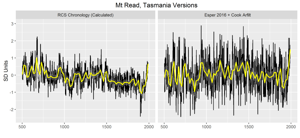
Figure 1. Mt Read versions (converted to SD units): left – RCS chronology calculated from Esper et al 2016 archive, edited to remove defects as described in Postscript; right – Esper et al 2016 reconstruction for Mt Read, extended prior to 1000AD with NOAA arfilt reconstruction (see discussion below).
Cook’s RCS Description and Age Profile Curve
A tree ring chronology is, in its essence, an estimate of an annual growth index after allowing for juvenile growth (since ring widths decline with age.) “Traditional” standardization fit a growth curve to each tree individually. But if growth rates varied between century, such techniques transfer variability over time to variability between trees. This type of problem is well known in statistics as fixed and random effects – techniques long advocated at Climate Audit – but these techniques are unfamiliar to tree ring scientists, who describe such phenomena in tree rings in coarse and artisanal terms.
Cook was keenly aware of the lack of low frequency variability in “traditional” standardization ( a technique that he had used in his original publication of Tasmanian data in 1991 and 1992). The issue also concerned Briffa, who, in two influential publications (Briffa et al 1991, 1992), advocated the use of a single growth curve for each site (rather than individual growth curves for each tree) as a means for retaining centennial variability, but, like Cook, being unable to express the issue in formal statistics. The single-growth-curve technique was subsequently labeled as “RCS” standardization. The technique has problems if the dataset is inhomogeneous between sites (as many are). There are numerous CA posts structuring chrobnology development in terms of fixed and random effects.
Back to Mt Read: Cook et al 2000 clearly and unambiguously stated that they used a single age profile curve (“RCS”) to allow for juvenile growth in chronology development:
In an effort to preserve low-frequency climatic variance in excess of the individual segment lengths, we applied the regional curve standardization
(RCS) method of Briffa et al. (1992, 1996) to the data.
Cook described his RCS technique in straightforward terms and (of considerable assistance for subsequent analysis) included a figure showing the age profile curve.
The RCS method requires that the ring-width measurements be aligned by biological age to estimate a single mean growth curve that reflects the intrinsic trend in radial growth as a function of age… The mean series declines in a reasonably systematic and simple way as a function of age. The simplicity of this ring- width decline with increasing age indicates that the RCS method may work well here…Therefore, a simple theoretical growth curve has been fit to the mean series. This RCS curve is shown in Fig. 2A as the smooth curve superimposed on the mean series.
Cook’s Figure 2A can be closely replicated from a quality-controlled version of the Mt Read dataset, as shown below, where my replication matches Figure 2A down to fine details. This match accomplishes three things. It confirms that differences between my RCS chronology and the archived Cook version do not arise from different age profile curves. Second, it also confirms the validity of my quality control editing for the defects and errors in the archive. While the edits were motivated by other inconsistencies, the age profile curve calculated on the data prior to quality control for stupid defects does not match. Third, the data is better fitted by a Hugershoff curve, a common form in dendro analysis (y= A+ B*x^D *exp(-C*x) ), than by a negative exponential (another common form). I accordingly used the Hugershoff fit in my calculation of the RCS chronology.
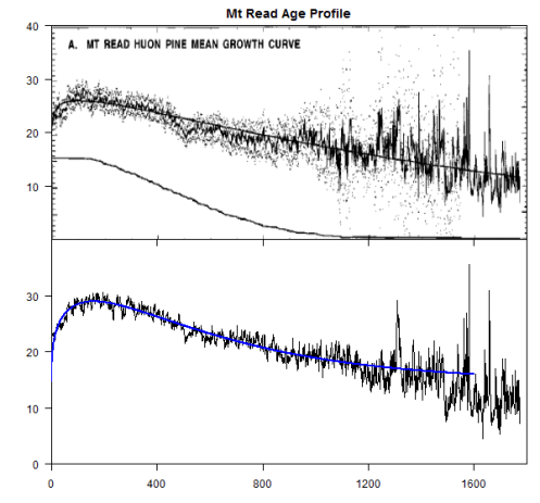
Figure 2. Mt Read age profiles. Top – from Cook et al 2000; bottom – calculated from archived measurement data. Blue- fit from Hugershoff curve y= A+ B*x^D *exp(-C*x). A slight discrepancy in fit on the far tail won’t effect results since so few measurements at this age.
Reverse Engineering
If Cook’s chronology wasn’t an RCS chronology, then what was it? Its lack of centennial-scale variability strongly suggests that it employed some form of fitting to each individual core. Cook’s first articles on Tasmania (Cook et al 1991, 1992) had employed smoothing splines – a technique which made it impossible to recover centennial variability, as Cook understood very clearly.
Another standardization technique employed at the time was (supposedly) “conservative” standardization with “stiff” negative exponential curves, a style of standardization used by Cook’s colleague, Gordon Jacoby – a technique which still standardized on individual cores (rather than one curve for the entire site). As a guess, I did a Jacoby-style standardization on the Mt Read data, comparing to the Cook et al 2000 Figure 3 chronology (archived as the NOAA “original” chronology) – see figure below.
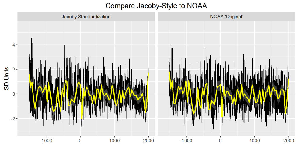
Figure 3. Mt Read versions. Left- using “traditional” standardization (negative exponentials for each core); right – NOAA “original”. The NOAA “original” version was illustrated in Cook et al 2000 Figure 3
It doesn’t match exactly, but the general similarity of appearance, combined with the dissimilarity to a freshly calculated RS chronology, convinces me that something went awry in Cook’s calculations. While he clearly intended to calculate an RCS chronology, I am convinced that the Cook et al 2000 chronology was calculated using some variation of “traditional” standardization (in which curves were separately fit to individual trees/cores), a conclusion supported by the lack of centennial scale variability.
Compare RCS Chronology to Mean Ring Width Series
The RCS chronology calculated in this post is closely related to the series of mean ring widths illustrated in Cook et al Figure 1A.
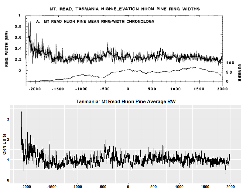
Figure 4. Top – Cook et al 2000 Figure 1A showing mean ring width; bottom – mean ring width series calculated from quality-edited measurement data.
Cook observed that his method (claimed to be RCS) had “removed some long-term growth” variation, but claimed (incorrectly in my evaluation) that it had preserved “much of the century-scale information”:
Comparing the mean series in Figs. 1A and 3A, it is clear that the RCS method has removed some long-term growth variations in the standardized chronology, but much of the century-scale information has been preserved.
This observation can be dramatically re-stated in light of the preceding analysis. The RCS calculation (this post) preserves virtually all of the long-term growth variation of the mean ring width series.
The “Original” and “Arfilt” Versions
Both Cook et al 200 and the associated NOAA archive contain two closely related versions of his chronology: the “original” version (shown in Figure 3) and the “arfilt” version (shown in Figure 7). To foreclose potential issues arising from differences between these versions, I’ve shown both variations against an RCS chronology in the figure below, this time showing values back to 1500BC (as in the NOAA archive), more than doubling the coverage shown in the first figure above.
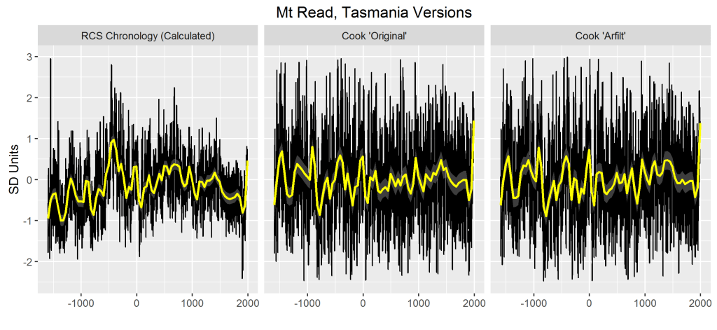
Figure 3. MT Read chronologies from -1500BC to 1991AD: left – RCS chronology (this post); middle: “original” chronology; right: “arfilt” chronology.
Relative to the RCS chronology, both the “original” and “arfilt” chronology appear very similar to one another and differ from the RCS chronology through their lack of low-frequency variability. In this view, one can discern a general correspondence in decadal features of the smoothed (yellow) version, while noticing that the Cook versions have flattened out high early values apparent in the RCS chronology.
Cook described the calculation of his “arfilt” chronology as follows:
Simple linear regression analysis was used to transform the Lake Johnston Huon pine tree-ring chronology into estimates of November-April seasonal temperatures. Prior to regression, both the tree-ring and climate series were prewhitened as order-p autoregressive (AR) processes… The tree-rings were modelled and prewhitened as an AR(3) process, with the AR order determined by the minimum AIC procedure (Akaike, 1974). The AR coefficients and explained variance of this model are given in Table 2. Note that the majority of the persistence is contained in the first coefficient (ARl = 0.397), which basically reflects an exponentially- damped response to environmental inputs such as climate. In total, this AR(3) model explained 21.8% of the tree-ring variance. In contrast, the November-April average temperatures were modelled as an AR(1) process that explained 10.5% of the variance (Table 2).
Reading this article today, it’s impossible to see any value added through the addition of the arfilt procedure to the “original” chronology, however this was actually calculated.
Even though the arfilt series is even further from an RCS chronology than the “original” chronology, this was the version used in both Gergis et al 2016 and Esper et al 2016. (This can be proven by digital comparison of the data.) Gergis et al 2016 contained 10 values for the arfilt series (1992-2001) not included in the NOAA archive and not supported by the the present measurement data archive, which ends in 1991. If the additional values arise from the inclusion of fresh tree ring data, it’s hard to understand why this data wouldn’t have some impact on the chronology up to 1991, but these values remain unchanged – even to the third decimal place.
Gergis et al 2016
As noted in the introduction, Gergis et al re-calculated tree ring chronologies from the underlying measurement data for all sites using an RCS variation (“signal-free detrending”) recently developed at the University of East Anglia:
All tree-ring chronologies were developed from raw measurements using the signal-free detrending method, which improves the resolution of medium-frequency variance…
The method has been presented as yet another recipe, with no attempt to place it in a broader statistical context.
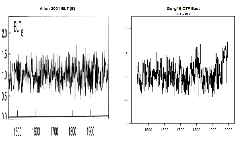
When the method was applied to tree ring sites in the Gergis network, it frequently resulted in much enhanced 20th century relative to previously published results, as, for example, for Celery Top East (shown below), where the published version had little centennial variability, but, as re-calculated by Gergis et al, had a very pronounced increase in the 20th century.
Figure 4. Celery Top East chronologies. Left- the (unarchived) BLT (East) chronology as illustrated in Allen et al (2001); right – the Celery Top East chronology archived in connection with Gergis et al 2016. The series name includes identifiers BLT and RFR, both sites discussed in Allen et al 2001. The difference between versions appears to arise from methodology, not data.
However, for Mt Read (and Oroko), Gergis used prior chronology versions, ostensibly for consistency with published results” – though such inconsistency had not troubled them in cases where they obtained elevated 20th century values. They described their choice of older versions as follows:
The only exceptions to this signal-free tree-ring detrending method were the New Zealand silver pine tree-ring composite (Oroko Swamp and Ahaura), which contains logging disturbance after 1957 (D’Arrigo et al. 1998; Cook et al. 2002a, 2006), and the Mount Read Huon pine chronology from Tasmania, which is a complex assemblage of material derived from living trees and subfossil material. For consistency with published results, we use the final temperature reconstructions provided by the original authors that include disturbance-corrected data for the silver pine record and regional curve standardization for the complex age structure of the wood used to develop the Mount Read temperature reconstruction (Cook et al. 2006).
It is evident that their decision to use a prior version of Mt Read was only made after examining results of the fresh chronology, which must have been similar to the results calculated above i.e. with elevated values in the first millennium and early second millennium. Such an election, only made after getting (presumably) adverse results is yet another example of data torture (Wagenmakers, 2011, 2012), for which Gergis’ proffered rationale (“consistency with published results”) is both flimsy and inconsistent with handling other series.
The version used instead in Gergis et al 2016 was, as noted above, identical to Cook’s arfilt series between 1000 and 1991. Gergis did not use values in the archive from prior to AD1000, but her dataset included 10 additional values (1992-2001). Presumably these additional values were provided by Cook, but, if they were calculated from additional data, one would have expected that earlier values would at least be somewhat impact (and not identical to three decimal places).
Esper et al 2016: Reconstruction and Measurement Data
Esper et al 2016 stated that they used the “most recent” reconstruction from each site. However, as noted above, the Tasmania reconstruction (values from 1000-1991 AD) in their archive ends in 1991 and is a shortened form of Cook’s arfilt reconstruction (archived at NOAA in 1998). Values before 1000AD were not archived for Tasmania, though earlier values were archived for many other sites.
Esper et al asserted that Cook’s Tasmania reconstruction had been produced from an RCS chronology, but this assertion does not appear to have been verified by Esper and/or other lead authors.
The Mt Read measurement data in the Esper et al 2016 archive appears to be more or less identical to measurement data archived at NOAA in 2002 (ausl024). Both contain many booby traps for the unwary – all of which ought to have been corrected long ago. Because of these defects, the archive is not readable using the R package dplR. Cook’s booby traps have several levels. Level 1: Cook’s measurement data contains in two different units. Each core segment has a trailing (final) value of either -9999 or 999; cores with a trailing value of 999 are in units that are 10 times larger. I do not recall any other measurement data archive which isn’t consistent. I don’t understand why this inconsistency isn’t tidied in the archive. Level 2: in all or nearly all measurement data archives, each core segment has a separate ID through adding a single-character suffix to the core ID. The end of each segment is marked by a trailing value of -9999 or 999. However, Cook’s archive contains multiple segments with the same ID, blowing up data assimilation. In my read program, problematic cores could be picked up by seeing if the core, after assimilation, still included a trailing value. There were about 15 such cores – in each case, I manually added a suffix to one segment of the core, thereby differentiating the segments to accommodate a yield. This took a lot of time to diagnose and patch. Level three: this was the trickiest. As a cross check, I examined the distribution of average ring widths by core segment and found that average ring widths for six cores (KDH89, KDH16B, KDH85, KDH61A, KDH64, KDH83) were about 10 times the average ring widths. Using the “native” values of the Esper archive, the age profile curve didn’t match the Cook et al figure. I concluded that the values for these cores in the Cook archive needed to be divided by 10 to make sense. I did this semi-manually and saved a clean measurement dataset, which I then applied. After this cleaning, the age profile match improved considerably. Note that these cores were all in early periods (mostly first millenium). Thus the editing of the data reduced first millennium values.
Conclusion
An RCS chronology calculated according to the stated methodology of Cook et al 2000 yields an entirely different result than that reported by Cook. In my opinion, Cook, like Gergis et al 2012, did not use the procedure described at length in the article – in Cook’s case, he did not use the RCS procedure described in the article as a method to preserve low-frequency variability. In my opinion, Cook’s chronology was most likely produced using a variation of “traditional” standardization that did not preserve low frequency variability.
Cook’s chronology has been used over and over in multiproxy studies: Mann et al 1998, Jones et al 1998, Mann and Jones 2003, IPCC AR4, Mann et al 2008; most recently, Gergis et al 2016 and Esper et al 2016. Despite its repeated use, one can only conclude that no climate scientist ever looked closely at Cook’s actual chronology, a conclusion circumstantially supported by the persistence of gross errors in the Cook measurement data, even in the Esper et al 2016 version, issued more than 20 years after the original measurements.
The actual RCS chronology for Mt Read has elevated values in the late first millennium and early second millennium. Gergis et al evidently calculated such a chronology and, in another flagrant instance of ex post cherry picking, decided to use the ancient Cook chronology, which turns out to have been erroneously calculated (like Gergis et al 2012, one might add). Use of the Mt Read RCS chronology and Law Dome series would obviously lead to substantially different results in the medieval period where Gergis only used two proxies.
Postscript
A reader pointed out that Allen et al (2014) reported an update to Mt Read. I should have taken note of this, but take some consolation in the fact that Esper et al 2016 didn’t take note of this update, despite claiming to have used the most recent series from each site and having a common co-author (Cook).
Allen et al took cores from 18 trees. Their reported chronology was not an RCS chronology, but a chronology based on fitting individual series – a technique that Cook had purported to avoid in order to preserve centennial variability. Allen et al describe the use of negative exponential curves, conceding that this technique “potentially loses some centennial time scale variability” relative to Cook et al 2000:
The updated chronology was constructed from the new samples and the previously crossdated material (Buckley et al. 1997; Cook et al. 2000) and is based on individual detrended series with a mean segment length greater than 500 years (Cook et al. 2000). All samples, including those previously obtained, were standardised… using fitted negative exponential curves or linear trends of negative or zero slope, with the signal-free method applied to minimise trend distortion and end-effect biases in the final chronology (Melvin and Briffa, 2008). The use of negative exponential and linear detrending preserves low-frequency variations due to climate consistent with the ‘segment length curse’ (Cook et al., 1995b), but potentially loses some centennial time scale variability that had been preserved in the Mt Read chronology based on regional curve standardisation (Cook et al. 2000).
My surmise is that the technique used by Allen et al is probably similar to, if not identical, to the technique that Cook et al 2000 actually used. The figure below compares Allen et al 2014 Figure 2C to the RCS chronology of this post. The two series are highly correlated, but the Allen chronology has flattened out the long-term decline of the RCS chronology.
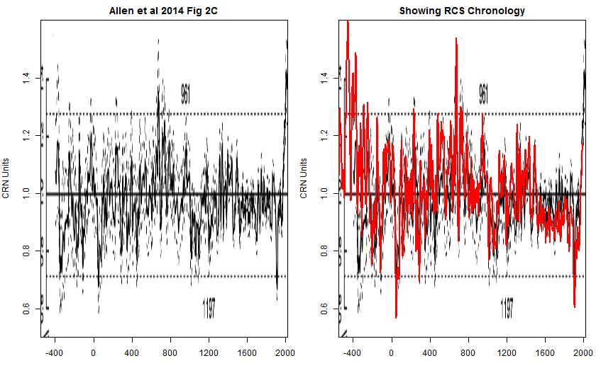
Figure ^. Left – Allen et al 2014 Figure 2C. Right – RCS chronology (this post) overlaid onto Allen Figure 2C.
Once again, it seems implausible that Allen et al 2014 did not first attempt an RCS chronology in order to directly update the Cook et al 2000 chronology, deciding to use an individually fitted chronology only after inspecting an RCS chronology. In addition, the start of their figure (400BC) neatly and perhaps opportunistically excludes high values in the immediately preceding interval.
References:
Allen et al 2014. Continuing upward trend in Mt Read Huon pine ring widths–Temperature or divergence? Quat Sci Rev. pdf
Cook et al 2000. Warm-season temperatures since 1600 BC reconstructed from Tasmanian tree rings and their relationship to large-scale sea surface temperature anomalies. Clim. Dyn. pdf
Gergis et al 2016. Australasian Temperature Reconstructions Spanning the Last Millennium. Journal of Climate.
Esper et al 2016. Ranking of tree-ring based temperature reconstructions of the past millennium. Quat Sci pdf.


220 Comments
“average ring widths for six cores (KDH89, KDH16B, KDH85, KDH61A, KDH64, KDH83) were about 10 times the average ring widths.”
???
Holy crap. Brilliant, meticulous work.
This is a real test of Cook’s character as a scientist.
Steve: I think that there is a greater issue regarding Gergis. There is strong evidence that their fresh version of the Tasmania chronology contained high medieval values, but they withheld these results “for consistency” with previous publications. Imagine the fate of a geologist who did this with drill results that failed to confirm prior results.
My point assumes a lot of back story.
I was giving Cook’s integrity the benefit of the doubt.
This episode simply adds to long list of sins for Gergis.
Found in the ‘sin soared’ file.
==========
“This is a real test of Cook’s character as a scientist.”
###
The test is whether Cook responds to this post. The geologist eventually has to answer, the dendros never need worry about that. But Steve McIntyre has done invaluable work here and that work will endure in the future while the work of the dendros joins Lysenkoism as a byword for the perversion of science.
snip – OT
Wonder if Michelson and Morley should have reported that the ‘aether’ existed for ‘consistency with previous results’.
Steve, is it possible that the ‘nine year addition’ comes from http://www.sciencedirect.com/science/article/pii/S0277379114003084
Allen, Cook et al 2014 QSR, from abstract,
“To date, no attempt has been made to assess the presence or otherwise of the “Divergence Problem” (DP) in existing multi-millennial Southern Hemisphere tree-ring chronologies. We have updated the iconic Mt Read Huon pine chronology from Tasmania, southeastern Australia, to now include the warmest decade on record, AD 2000–2010, and used the Kalman Filter (KF) to examine it for signs of divergence against four different temperature series available for the region. Ring-width growth for the past two decades is statistically unprecedented for the past 1048 years…..”
The full paper is available here. There’s some interesting stuff in the paper. Cook is the second author, and for some reason, they decided:
“All samples, including those previously obtained, were standardised using fitted negative exponential curves or linear trends of negative or zero slope, with the signal-free method applied to minimise trend distortion and end-effect biases in the final chronology. The use of negative exponential and linear detrending preserves low-frequency variations due to climate consistent with the ‘segment length curse’, but potentially loses some centennial time scale variability that had been preserved in the Mt Read chronology based on regional curve standardisation. Because our tests of divergence are based only on the outer 100 years of the chronology concurrent with meteorological
data, the way we have standardised the chronology here versus the way done by Cook et al. (2000) should not have any impact on the possible detection of divergence in the Mt Read chronology”
They also have a lot of discussion around the divergence problem, they are evaluating it as a “time dependence”. They have a test that plots divergence over time. And they have this in the conclusion:
“it is abundantly clear that the conclusion that inferred ring-width-based temperatures over Tasmania and southeastern Australia for the past decade and a half have been higher than for any other period in the past 1000 years is a conditional one. It is conditional on the assertion that the relationship between temperatures and ring width has remained sufficiently stable over time”
“It is conditional on the
assertionassumption that the relationship between temperatures and ring width has remained sufficiently stable over time”Fixed. 😉
Thanks for drawing this article to my attention. I’ve added the following section to the post:
Postscript
A reader pointed out that Allen et al (2014) reported an update to Mt Read. I should have taken note of this, but take some consolation in the fact that Esper et al 2016 didn’t take note of this update, despite claiming to have used the most recent series from each site and having a common co-author (Cook).
Allen et al took cores from 18 trees. Their reported chronology was not an RCS chronology, but a chronology based on fitting individual series – a technique that Cook had purported to avoid in order to preserve centennial variability. Allen et al describe the use of negative exponential curves, conceding that this technique “potentially loses some centennial time scale variability” relative to Cook et al 2000:
My surmise is that the technique used by Allen et al is probably similar to, if not identical, to the technique that Cook et al 2000 actually used. The figure below compares Allen et al 2014 Figure 2C to the RCS chronology of this post. The two series are highly correlated, but the Allen chronology has flattened out the long-term decline of the RCS chronology.
Figure ^. Left – Allen et al 2014 Figure 2C. Right – RCS chronology (this post) overlaid onto Allen Figure 2C.
Once again, it seems implausible that Allen et al 2014 did not first attempt an RCS chronology in order to directly update the Cook et al 2000 chronology, deciding to use an individually fitted chronology only after inspecting an RCS chronology. In addition, the start of their figure (400BC) neatly and perhaps opportunistically excludes high values in the immediately preceding interval.
Wow. A lot of work, Steve. Thanks!
As usual, you put the so-called “professional” climate scientists to shame. Good grief.
Cheers — Pete Tillman
Professional geologist, advanced-amateur paleoclimatologist
Excellent work again. This is what real replication look like. My thanks and appreciation.
Perhaps “consistency with published results” doesn’t refer to proxy consistency with the original authors’ publications. Rather, the G2016 reconstruction should resemble that of G2012. 😉
“When the [new] method was applied to tree ring sites in the Gergis network, it frequently resulted in much enhanced 20th century relative to previously published results, as, for example, for Celery Top East”
Any investigation into this new method on the horizon? Just asking.
Great work, Steve.
As ever we are reminded of climate scientists blatant and so far unchallenged by the scientific community, explanation of data torture;
D’Arrigo: “you have to pick cherries if you want to make cherry pie”
Esper: “the purpose of removing samples is to enhance a desired signal, the ability to pick and choose which samples to use is an advantage unique to dendroclimatology”
Says it all.
Thanks Steve for an important analysis of Cook’s Mt. Read TR data sets.
The implications are staggering. All the papers using the improperly reconstructed data (without RCS) must be re-evaluated or discarded.
Thanks Anon for the Allen-Cook(2014) paper on the “Divergence Problem” (DP)
in relation to temperature. It seems like so many of these papers go ahead with a reconstruction, (past projection,) knowing the underlying methodological assumptions are unsettled. But the DP is not just an uncorrected age-growth bias or mistaken spliced thermometer record, DP tears at the fundamental assumption of the proxy’s validity at modern temperature levels.
This is a huge issue because if modern decade warmth levels are “unprecedented” there is no ability to demonstrate this unless the DP can be unequivocally linked to an non-temperature growth limiting factor that in itself assumed unprecedented (anthropogenic). Obviously the dendros must be studying ozone hole and every type of pollution like mad.
Allen-Cook(2014) asserts a non-strict DP for Mt Read where its correlation decouples not only in the recent 15 years but also at past times. Also this: “Unlike the decoupling first observed by Jacoby and D’Arrigo (1995) in which ring widths underestimated temperature in recent decades, the Mt Read ring widths overestimate warm season temperature for the past two decades.” But they admit that could be due to bad data or processing. Good for them.
“All the papers using the improperly reconstructed data (without RCS) must be re-evaluated or discarded.”
Yeah, we can count on that. NOT.
It’s pay-walled to me. Did they even discuss the possibility of CO2 fertilization?
Charles, the paper autodownloads to a pdf for me in Windows. Allen-Cook(2014) refers to CO2 fertilization several times citing LaMarche(1984), Brienen(2012), and Gedalof(2010). None cite Loehle(2009)— Sorry Craig (I found it searching: loehle 2008 divergence).
Craig, do you think Mt Read’s unprecedented growth rate for past 15-20 years cited by Allen et al could be CO2 limiting factor elevation, in other words, CO2 fertilization?
Brienen(2012) felt that sampling bias for picking larger, healthier trees was more significant than CO2 bias. It suggested using random sample selection. (We could have told them that.)
Craig,
Regarding the warming in Scandinavia, has the elevation of the treeline increased?
Jeff Norman: There has been elevation of the treeline, and I think it is increasing.
From 1909 Norway: Scientists concludes that treeline is elevated to a level of 1930ies.
And not very good match between models and observation.
Rate of forest advance and tundra disappearance. From Annika Hofgard 2015:
• Yes, trees and shrubs are moving up and north, but ……..
• Where – local to regional perspective
• Why – causal background (non-climatic drivers can
dominate)
• Mismatch between predictions and observations
• Mismatch between results based on experiments vs.
natural (both rate and species-specific responses)
• Rate of advance – not km but meters/year
• Modelled tundra loss of 40-50% – a serious overestimate
• Multi-site analyses are needed to refine regional and
circumpolar forest advance scenarios
• If not – misleading interpretations regarding rates of
climate-driven encroachment will prevail
• Model-based rate scenarios may cause management
failures.
And – there were big forests in highlands of Norway 7000 years ago that have no trees now (only Mountain birch).
Once the scientist doing temperature reconstructions can except (incorrectly) the post fact selection of proxies, the remaining data torture that is frequently applied falls within the boundaries of post fact selection.
Thanks, SteveM for the good review of the basis for the various methods used to extract tree ring response from ring width that varies with tree age. Without a consensus on a given method the scientists doing reconstructions are evidently allowed to use whatever method serves their purposes.
Thanks, Steve, for a very impressive piece of detective work and analysis. Yet more evidence that something is very wrong in the dendrochronology field.
Correction: I meant dendroclimatology, of course.
Mr. McIntyre: “Presumably these additional values were provided by Cook, but, if they were calculated from additional data, one would have expected that earlier values would at least be somewhat impact(ed) (and not identical to three decimal places).” I am intrigued by this. Are you suggesting that a splice of instrumental data was used here? Or, more basically, do you have a possible explanation for this strange situation?
Steve: not suggesting instrumental data and doubt it. I really don’t know.
Steve,

After the corrections you describe, my next focus would be on the relation of tree data to temperatures, the calibration stage.
I have actually seen Mt Read at close range. Few others have. It sits about where the Tasmanian west coast sub-climate meets the different east coast sub-climate.
The climate difference cannot easily be described by the recorded temperatures from near to Mt Read, for there are few stations. Here is a rough summary of those within say 100 km of Mt Read. Although there have been mines nearby since the late 1800s, there are few public BOM records earlier than the 1960s. That is, we do not have many (any) useful temperature records for the period before CO2 is alleged to have changed global climate and possibly tree growth.
Here is a snapshot of those BOM records as at 2007, with start and finish dates and position in lats and longs. Most to all of these records have slabs of missing data and are not useful.
So, temperature calibration is not good over the 0-100 km range. Over the whole of Tasmania, an island about 300 x 250 km in size, the longer term records are at Hobart and Launceston, some 200 km and 135 km from the target at Mt Read. Launceston in particular has several local weather stations used at various time intervals. It is hard to extract a composite picture and maybe it is not worth the effort because only the brave would claim the climate at Launceston to be similar to that at Mt Read. So, to calibrate with temperatures, Cook and others have looked at proxies of sea surface temperatures west of Mt Read, at Antarctic temperatures (which have hardly changed) and even to Asian monsoon regions.
Conclusion – what is the value of a publication as a temperature proxy when there are such difficulties relating tree properties to known temperatures?
Geoff:
the value os that one gets a times series with a particular pattern of variance, another tool in the box to employ when curve fitting.
The fact that there is no way to calibrate it to temperature with local records is a strength, not an impediment.
This means you can take your squiggles, and calibrate it to whatever you wish.
The huon pines at Mt. Read are an interesting bunch, they are all male and have the same DNA, it is thought they are clones of a tree about 10,000 yrs old that has been reproducing vegetatively since then.
http://www.apstas.com/Mt__Read_Huon_pine.html
a very interesting link that I commend to readers
“Because the rings vary with the climate at the time, and particularly with temperature, they give a good indication of how the climate has varied over that time. Of interest in this record is the clear indication of climate warming since the 1960’s.”?
really?
Another thought…since all the pines are genetically identical, one wonders just what the variance in phenotypic expression across all of the clones looks like?
same tree, almost identical location….same climate (same microclimate)…..
just wondering.
“Because the rings vary with the climate at the time, and particularly with temperature”
Isn’t this just the same ol’ assertion?
Andrew
that was a throw away line in a piece that mainly dealt with the genetics of the population of pines. a quick read.
worth the time.
Steve, the article says Mt Read Huon Pines chronologies are over 4000 years old. Have you found any from 2000BC? Would they not give better indications of the proper corrections to preserve low frequency?
A google books view of “Australian Rainforest Woods, Morris Lake, 2015 (CSIRO Publishing) mentions on page 115 a 7000 year long chronology for Huon wood on Mt. Read (by Mike Peterson – senior forester).
“The huon pines at Mt. Read are an interesting bunch, they are all male and have the same DNA, it is thought they are clones of a tree about 10,000 yrs old that has been reproducing vegetatively since then.”
Reminds me of the ents losing the ent wives.
Tolkien’s intuition. I’d trust that ahead of some notables in the field.
Finally, a rival for the most important tree in the world (Yamal).
“For consistency with published results” as a reason is pretty mind-boggling in a supposedly scientific paper. How could any errors ever be corrected if this was the approach taken to them?
And, while Gergis has clearly identified herself as a non-scientist with this phrase and many others, where are Cook and Allen and Esper and all their co-authors? Do none of them actually care about getting something like the correct answer out of these datasets? Do they accept these findings or not?
“The use of negative exponential and linear detrending preserves low-frequency variations due to climate consistent with the ‘segment length curse’ (Cook et al., 1995b), but potentially loses some centennial time scale variability that had been preserved in the Mt Read chronology based on regional curve standardisation (Cook et al. 2000).”
I have been puzzling over this claim for a while. I have the gnawing suspicion, borne of reading too much climate science, that the evidence for this claim is that the use of RCS in a direct comparison to individual series standardization leaves bigger wiggles. But are the wiggles bigger because RCS “preserves variability,” or because the magnitude of growth standardization error is greater if you apply a regional curve?
From the link above in a Ron Graf post about tree selection and the biases that result from those practices we have:
Click to access brienen_gbc12.pdf
My blockquote should have included only the firat paragraph.
Yes, Ken, its clear that they are aware of the problems (and the failures) of tree ring climatology and this fact starkly underscores their lack of participation here. They read the posts and the comments here, I have no doubt.
I doubt that post-1950 tree-ring data can be compared with earlier tree ring data. I read these posts with interest but often limited comprehension, so perhaps I am off base here. But bear with me on this. Recent studies have shown a worldwide greening of vegetation which is attributed to rising levels of carbon dioxide. https://wattsupwiththat.com/2016/04/27/nasa-carbon-dioxide-fertilization-greening-earth-study-finds/
So I think it is safe to say that rising levels of carbon dioxide are changing the way plants grow. And wouldn’t this at least imply that rising levels of CO2 would have an effect on the growth of trees and their annual rings? And wouldn’t this effect, whatever it is, be progressively greater as CO2 increases? So it seems to me that post-1950 tree rings would be “contaminated” with a CO2 effect that is increasing through time. Thus I suggest that post-1950 (or whenever you want mark the beginning of increase in atmospheric CO2)tree rings cannot be compared to tree rings laid down in the earlier CO2-stable atmosphere until the CO2 effect can be characterized and quantified.
TedL:
Fertilization is a bit OT, but see this:
“The annual growth of trees, as represented by a variety of ring-width, densitometric, or chemical parameters, represents a combined record of different environmental forcings, one of which is climate. Along with climate, relatively large-scale positive growth influences such as hypothesized `fertilization’ due to increased levels of atmospheric carbon dioxide or various nitrogenous compounds, or possibly deleterious effects of `acid rain’ or increased ultra-violet radiation, might all be expected to exert some influence on recent tree growth rates. Inferring the details of past climate variability from tree-ring data remains a
largely empirical exercise, but one that goes hand-in-hand with the development of techniques that seek to identify and isolate the confounding influence of local and larger-scale non-climatic factors.”
This is from the same 1998 paper I quoted above:
Click to access 43XA8LK6PCMVMH9H_353_65.pdf
so workers in this field are well aware of these confounding factors. That is not the same as saying that they have developed good methods for dealing with them!
TedL:
Your getting caught up on the reasons why the divergence might be real, but you are ignoring why it might not even matter.
The first step in determining whether a thing is a proxy for something else should be to detail why and under what conditions a person thinks that a thing being measured is a good proxy for something else. You then need to sample and see if it correlates. If it doesn’t, figure out why and refine your sampling criteria.
You don’t sample a bunch of stuff, then use the ones that correlate well. Must less sample it, see that part of it correlates and another part doesn’t, then just throw out the part that doesn’t.
Are the trees a proxy for temperature or just a coincidence for a number of years? If it is a coincidence, then there is no reason to even look at a 1950 or whatever year divergence as it shouldn’t even be used as a proxy.
MattK
Au contraire!
The protocol you outline above (and denigrate, BTW) is exactly what one does.
/sar
Steve, does the TR data contain information on the cambian (life) age of the samples? In other words how do we know that the 3000-yr chronology is not a truncated version of a 4000-yr or 7000-yr chronology? And doesn’t one need to know that in order to apply the RCS correction?
Steve,
I note that you defend your repeated use of the term “data torture” on the grounds that it is a well defined term in something called “statistical commentary”, whatever that might be. Indeed you define it as a “Technical term”:
” The term “data torture” is a term that is used in statistical commentary – I cited Wagenmakers. It has a technical meaning that precisely fits Gergis et al 2016.”
Technical terms, like entropy, chemical equilibrium, or anthropogenic global warming, have quite strict definitions that are understood by the community of technical specialists who use the terms. Indeed it would have to have a precise definition in order to “precisely fit” a particular phenomenon. Would you care to provide, preferably by reference to an appropriate dictionary of technical terms, a clear definition of the term? The fact that you only seem to be able to cite one individual, by the name of Wagenmakers, as using this “technical term”, suggests it does not have any such “community acceptance”, whether among “statistical commentators” or anywhere else.
Google is your friend.
Ronald Coase, economist and previously the Clifton R. Musser Professor Emeritus of Economics at the University of Chicago Law School, is the source of the most popular use of the phrase, brought into the cultural lexicon in the early 20th century: “If you torture the data enough, eventually it will confess.”
Which, of course, is exactly what Gergis did.
Coase was also awarded the
The Sveriges Riksbank Prize in Economic Sciences in Memory of Alfred Nobel”,
the prize commonly referred to as “the Nobel Prize in Economics” in 1991.
What would he know about applied statistical analysis, after all?
David E,
So if a word or phrase is in “the cultural lexicon” are you saying that makes it a technical term? Are, for instance, “motherf****r” or “asshole” a technical term. They are both indubitably part of the cultural lexicon.
The problem is that Steve is using the “technical term” argmument as a justification for what, at face value, is an insult, especially when he uses it repeatedly.
its an accurate description of the statistical analysis to which Gergis subjected data.
In all of your bleating and moaning, I fail to discern any critique of Steve’s analysis of Gergis’ indefensible practices.
Here we go: another yet apologist for the inexcusable shows up to quibble over the definition of a term, which in this case is clear, precise and altogether appropriate.
Bill h,
“As I’ll show below, it is hard to contemplate a better example of data torture, as described by Wagenmakers, than Gergis et al 2016.” – Steve McIntyre
Can’t be clearer. Go read the links to Wagenmaker that Steve McIntyre provided. These will serve much better than any dictionary to define and illustrate the abuses of statistical techniques known as “data torture”.
You should not expect any authoritative definitions of “data torture” to be issued by the tree ring climate community.
Craig, and what evidence is there in my post that justifies your attack on me.
I thought scientists were supposed to draw conclusion s based on evidence.
Easy there, Bill. What evidence was there in Craig’s response that you were being “attacked”? This is a site for informed and spirited discussion. Better develop a little thicker skin if you’re going to be that easily rattled by a couple of pointed questions.
G.Holcombe,
Sorry, but saying that I “think it is ok to keep doing statistical tests with different methods until you get a result you like? And ok to include or exclude data depending on how it affects the answer?” does look like an attack on my integrity.
Also in what way is Craig’s remark “informed”, to use your characterisation of this website. What evidence informs Mr. Loehle’s conclusion about what I think is “OK”?
bill h, it serves very well as a term for discussions. The phrase encompasses and represents violations of approved statistical techniques, as described in Steve’s links to Wagenmaker (did you avail yourself of those links?). Used in such a manner, it is a valid term. Yes, its use by a Nobel laureate in the same context authenticates its use by Wagenmaker.
The tree ring climate community would benefit enormously by a study of Wagenmaker and Steve McIntyre’s examples of “data torture” in the Gergis et al 2016.
Erm, David E. I suggest you have look at some of those “examples”, before citing them as evidence.
Also, where have I claimed ignorance of the term “data torture”? Again, a bit of a non-seq
bill, the monologues intersecting must both be in good faith to constitute a conversation. Yours is lacking something essential.
===========
bill h:
I cited the number of hits for that phrase to make the plain that it is widely used in peer reviewed articles published by those who practice applied statistical analysis,
that its been the subject of quite a bit of research,
and to show that if you are indeed ignorant of the term, or the application of it to a myriad of untenable practices, that you aren’t really qualified to maintain that your opinion on this issue is an educated one, thats all.
I suggest you look at a few screens worth of relevant research, just to familiarize yourself, before you go and waste others’ time again.
“I queried “data torture”, google scholar returned around 220,000 results.
heres the link:
https://scholar.google.com/scholar?hl=en&q=data+torture&btnG=&as_sdt=1%2C39&as_sdtp=”
If you use “data torture”
96 results.
not 220K
I replicated your search. good faith.
I got 220K, as you did
BUT
as I noted, they were mostly about ACTUAL torture
using a quoted “data torture” yeilds 96
Like I said.. do the math on 96/220000
First page includes
[BOOK] Torture and its consequences: Current treatment approaches
M Basoglu – 1992 – books.google.com
… Victoria 3166, Australia © Cambridge University Press 1992 First published 1992 Printed in Great
Britain by Bell and Bain Ltd., Glasgow A catalogue record for this book is available from the British
Library Library of Congress cataloguing in publication data Torture and its …
Cited by 192 Related articles All 3 versions Cite Save More
[CITATION] Torture: does it make us safer? is it ever OK?: a human rights perspective
K Roth, M Worden, AD Bernstein – 2005 – Human Rights Watch
Cited by 5 Related articles Cite Save More
Create alert
Page 2
Is torture reliably assessed and a valid indicator of poor mental health?
M Hollifield, TD Warner… – The Journal of nervous …, 2011 – journals.lww.com
… Descriptive data about the 3 groups are provided below. The TEQ was transformed to
dichotomous data (torture vs. nontorture) by combining the nontorture war trauma and no
war trauma groups into 1 nontorture group where required for analyses. …
Cited by 4 Related articles All 8 versions Cite Save
By page 5 it looks like this
https://scholar.google.com/scholar?start=40&q=%22data+torture%22&hl=en&as_sdt=1,5
Here you go
https://scholar.google.com/scholar?hl=en&q=%22data+torture%22&btnG=&as_sdt=1%2C5
96 results
not 220,000
Somebody learned to search from gergis or maybe it was just your typo.
Bill,
“… Sorry, but saying that I “think it is ok to keep doing statistical tests with different methods until you get a result you like? And ok to include or exclude data depending on how it affects the answer?” does look like an attack on my integrity. …”
Actually, that series words is terminated with a question mark? That is, you were asked a question. No one attacked you, though you could perhaps understand that your prior comment read in a rather “post-normally” permissive mode, and that some might view such permissiveness as a less than rigorous approach to gaining understanding. Wagenmaker is far from the only individual to use the term. I heard it in use by Peter A. Griffin, who taught some of my stat classes in ’70s. In fact, “data torture” is rather obvious simile when you look at statistics used on selectively biased data to support prior assumptions. Dr. Griffin once described a study we were required to read and criticize has having been conducted by a “data Torquemada.”
So, because a nobel laureate uses a phrase it automatically becomes a “technical term”
Bill,
Also see Mills, 1993 published in the NE Journal of Medicine:
http://www.nejm.org/doi/pdf/10.1056/NEJM199310143291613
no…
its your abject and proud ignorance of the term, its provenance, its history and its meaning thats somewhat irritating Bill.
Why not go to google scholar and search for “data torture”
get back to us?
here: i did the heavy lifting for you:
I queried “data torture”, google scholar returned around 220,000 results.
heres the link:
https://scholar.google.com/scholar?hl=en&q=data+torture&btnG=&as_sdt=1%2C39&as_sdtp=
that you seem to be unaware of this term, and its applicability to subject at hand says a lot about you bill, and not much of it is good.
“I queried “data torture”, google scholar returned around 220,000 results.
heres the link:”
I did the same thing.
However, I actually looked through pages of cites.
there were only a few that referred to data torture, the vast majority were about TORTURE
as in hurting people.
so… dig a bit deeper
When I googled “‘data torture'” with bounding quotation marks, nearly all the retrievals were relevant to data torture.
Steven Mosher
I did: https://climateaudit.org/2016/08/16/re-examining-cooks-mt-read-tasmania-chronology/#comment-770649
Did you not see that one?
From the Devil’s Dictionary by Ambrose Bierce:
Pen- an instrument of torture wielded by an ass.
Thank you Steve.
Mosh. youre simply not arguing in good faith.
a multitude of the citations returned by the query “data torture” submitted that way, with the term in quotation marks are on point.
Youre really grasping at straw men now.
You know what the term means…
Anyone who has done any work in the field does as well.
there are thousands of citations for that term.
Why you would choose this battle field to stand and fight is incomprehensible.
More to the point:
Do you endorse the practices that Gergis employs?
“Thank you Steve.
Mosh. youre simply not arguing in good faith.”
I used your link.
https://scholar.google.com/scholar?hl=en&q=%22data+torture%22&btnG=&as_sdt=1%2C5
96 results
not 220k
What’s your point, Mosh? That 96 retrievals is not enough? That more is needed?
I don’t see why you saw fit to complain in the first place. Piddling criticism. One the links here is to a 2007 CA post. In your comments you blew hot against the “tree ring circus” (your words).
How you have changed.
The google search for “data torture” reveals a number of papers. One of thse papers on “data torturing” has 173 citations. So the assertion that there are only 96 results for the concept appears to be refuted – 173 citations to one paper on the concept
I reviewed literature on data torture long ago and have notes on many interesting articles. I found some by Google and some by tracing citations.
I fail to see why it is relevant whether there are 96 google references vs 220,000 for the more general terms “data” “torture”, both of which are common words. I didn’t say that there were 220,000 references to “data torture”, so I’m puzzled at the point.
As mentioned before, I find the concept of “data torture” to be useful term to note poor statistical practice, especially in the context of motivated researchers, without implying the additional baggage of misconduct and/or fraud. I distinguish such usage from use of the term as mere abuse. I completely fail to understand why anyone would object to such usage.
In my recent comments on Gergis, I’ve generally tagged the usage with a citation to Wagenmakers (2011,2012), even using the additional qualification “sensu Wagenmakers” on occasion. As previously pointed, I submit that Gergis’ screening in Gergis 2016 is a classic example of data torture as described by Wagenmakers. I don’t see how anyone can reasonably contest this point, nor has anyone done so thus far.
Steve:
This is my fault.
I ran the query without quotation marks, and cited the number of hits google scholar returned…
Of course some are not relevant, however, many are.
Some here chose to pick a couple of non relevant hits, and focus on them, while ignoring the large number of relevant cites, the provenance of the quote and its applicability to the situation at hand.
Cherry picking?
IDK.
Its sad and interesting just what some choose to focus on.
BTW, I reread you post detailing your own efforts to update some tree ring chronologies.
The hardships you endured while attempting to access remote sites.
The logistics involved in bringing heavy equipment to the site, as well as the excellent documentation of the trees previously sampled, a practice which no doubt made it so much easier for you to identify those trees.
I should be clear.
I appreciate the work Mosh has done for all of us.
However it is obvious that he hasn’t absorbed the most fundamental concepts that undergird the entire enterprise of applied statistical analysis.
The results of this failure can be seen across disciplines, for example, the financial crisis caused by bundling collateralized debt obligations (it was argued that the individual mortgages’ behavior was independent of each other, a laughable construct once made explicit).
Mosh’s expertise with R doesnt mitigate his lack of concern for practicing sound statistical analysis.
You just have to love it.
Google ignores delimiters. In a Google search, Google applies their own version of what their programmers prefer you search on.
Bing, however, still allows delimiters.
Using Bing and the following search:
+”data torture”
returns 3,820 results.
First in line is Climateaudit’s “Joelle Gergis, Data Torturer”; but is followed by many diverse sources.
Mosher, as is becoming tediously common, seems to be more interested in raising pointless objections, than in addressing anything of substance. Yes, data torture (without quotations) will bring up many hits involving actual torture. However, Mosh’s response (change the search to “data torture”) is silly as it will exclude many relevant results. “Data torturing” yields an additional 265 hits on google scholar (probably some overlaps). “Torturing data” is 180. “Torture the data” is 634. I think it hard for anyone (including Mosh and bill h) to sustain an argument that it is not a term of art in the statistical literature.
If bill h is not just trolling and is genuinely interested in an answer as to what is data torturing, there is a good description in one of the first google hits from the famed NEJM: “IF you torture your data long enough, they will tell you whatever you want to hear” has become a popular observation in our office. In plain English, this means that study data, if manipulated in enough different ways, can be made to prove what-ever the investigator wants to prove. Unfortunately, this is generally true. Because every investigator wants to present results in the most exciting way, we all look for the most dramatic, positive findings in our data. When this process goes beyond reasonable interpretation of the facts, it becomes data torturing.”
“I fail to see why it is relevant whether there are 96 google references vs 220,000 for the more general terms “data” “torture”, both of which are common words.”
“I cited the number of hits for that phrase to make the plain that it is widely used in peer reviewed articles published by those who practice applied statistical analysis,
that its been the subject of quite a bit of research,”
Seems like 96 or 220K is relevant 220K is rather Yamal like
More funny is that I use the very link provided to do the search and get condemn for having bad faith.
too funny
Really Mosh:
this is beneath you.
I provivded a link, one that returned hundreds of thousands sites.
Now, be a big boy and refine my query if you dont wish to wade through the larger body of results.
As if my point is any less valid if there are only tens of thousands of citations?
Geez mosh, its just sad.
You present a selected subset of three responses and attempt to argue that the term isnt commonly used in peer reviewed literature?
That it doesnt exist in the current lexicon?
That my contentions were in some way incorrect?
mpainter, your non-sequitur responses are becoming rather trying. I am reminded of Rebecca West’s rather cynical definition of “conversation” as “an intersection of monologues”. To re-quote Steve:
” The term “data torture” is a term that is used in statistical commentary”. “It is a technical term”.
So, it’s a technical term drawn from the “statistical commentary community”. Your comment about the “tree ring community” has no relevance
Sorry, the second sentence of my quote is incorrect. It should read “It has a technical meaning”, NOT “It is a technical term”.
The post in large part is addressed to the tree ring climate community. My comment was indeed revelant.
Where is ATTP, I wonder.
Also, bill h, please correct me if I’m wrong, but you presumably agree with the rest of my comment above, as you did not demur. I copy it below for your convenience.
Posted Aug 19, 2016 at 11:34 AM | Permalink
bill h, it serves very well as a term for discussions. The phrase encompasses and represents violations of approved statistical techniques, as described in Steve’s links to Wagenmaker (did you avail yourself of those links?). Used in such a manner, it is a valid term. Yes, its use by a Nobel laureate in the same context authenticates its use by Wagenmaker.
bill h: Your subtle ploy was too clever for us. The old “false AND immaterial remark” ploy, to get us arguing whether it’s more untrue than pointless or more pointless than untrue. And asking the host to do your homework, nice touch. Sorry that last part failed for you. Oh, first part failed too. Look at the bright side, you’re good at failing. Just thought I’d help you recognize an attack
LOL, here is another technical term for bill h, “cavil”. Would I be cavalier to call bill h a caviler.
How about ‘draws conclusions that are extremely non-robust to arbitrary methodological choices’.
bill h, you need to correct your mis-attribution in this comment. Steve posted the words “technical meaning”, and your comment above falsely attributes to him the expression “technical term”.
Thus your fuss about use and definition is baseless.
Somewhat loath to continue to kick this can down the road, but the man did ask for a reference in a dictionary of technical terms or some such.
I note that the Data Archives section of the Encyclopaedia of Biostatistics (which this what this is basically all about) says:
“Finally, the requirement to provide original data is one protection against the production of findings based on a particular statistical approach to the data – findings produced by what is commonly called “data torture” and the actual fraudulent invention of results.”
Davey Smith, G. 2005. Data Archives. Encyclopedia of Biostatistics. 2.
Can we move on?
TY HAS.
Actually David I should have added a h/t in your direction. All I did was add quotes around the phrase in your google scholar search and it found itself.
billh, I would just suggest that the term is well defined in the statistical literature. The real question is whether or not you disagree with SteveM’s characterization of Gergis et al. If so, please tell us why. If not, then you are just quibbling.
Tales of Horror from Ivory Towers, vintage 1980, mentions “data torture.”
Steve: an article that acknowledged with thanks comments from my former golf adversary, George Stigler.
you golfed with Stigler?
now Im impressed.
Steve: Stigler used to take summer vacation on Lake Rosseau in Muskoka, Ontario. He played at Muskoka Lakes Golf Club, as did my family. When I was 13 or 14, I was playing with some friends and were playing behind Stigler and his friends, who were taking forever. On the 11th hole, a par five, we got tired of waiting for them and hit our second shots before they finished putting out. I hit a really good shot and it run onto the green about 10 feet from the hole inside where they putting out. I was really excited because I had a chance for an eagle, which I’d never had. However, Stigler picked up my ball and threw it into the woods. I knew who he was because I’d caddied for my father in a club tournament against Stigler, who’d beaten him. By chance, I played against Stigler in the club tournament later in that summer. Trounced him. He was pretty annoyed because I was then pretty young.
Mike Spence, another Nobel laureate, was an older contemporary of mine at high school in Toronto.
I am less impressed with Stigler now than before I knew this
😉
Im glad you got the chance to beat him.
A slow, poor golfer shouldn’t ruin some kid’s excellent round.
It is a certain kind of guy who takes it upon himself to teach someone else’s 13 year old boy a lesson.
Am reminded of Stigler’s Law of Eponymy which holds that no scientific discovery is named after its original discover. (Stephen Stigler–George’s son) At first blush it occurred to me that the Mann Hockey Stick runs counter to this, then I remembered the “scientific” qualifier.
You say:
On the contrary, if I were to characterize the literature using the phrase, I would say that the term is used somewhat differently by different people. I have never said that “date torture” is a “well defined term”. That is a fabrication on your part.
Precisely because there is no uniformity of usage, I cited Wagenmakers (2011,2012), which used the term to describe a variety of disapproved statistical techniques, arguing that Gergis et al 2016 amply met the criteria for data torture sensu Wagenmakers – an observation that you have not directly contested.
Your assertion that I “only seem to be able to cite one individual, by the name of Wagenmakers, as using this “technical term”” is simply untrue. I could have cited numerous other uses of the term “data torture”, but was writing a blog post about Gergis et al 2016, not an exegesis of the term “data torture”. Other uses can readily be found through Google and by tracing various references.
While I do not have time to fully canvass the uses of the term “data torture”, I think that the term is particularly useful in characterizing poor statistical practices (of which there are manifold types), which one does not wish to characterize as fraud or misconduct (though characterization as data torture does not exclude). Wagenmakers 2011, 2012 gave a variety of examples.
Clarity.
Charity.
Two foxes shot. That was fun to read.
Gergis’s response on her paper gergis 2012 and gergis 2016 was that the only error was the incorrect reference to de trended data instead of trended data. Her claim was that correcting for the “typo’ / “missidentification” of the method was the only error and that amateur Bloggers were making a mountain out of a mole hill.
https://theconversation.com/how-a-single-word-sparked-a-four-year-saga-of-climate-fact-checking-and-blog-backlash-62174
If I am not mistaken, the substantive issue is the use of certain proxies which provide the “desired result and the exclusion of proxies which contradict the desired result.
Her argument (which includes complaints of blogger gender bias) is more of a case of trying to hide the mountain with a mole hill.
I just read that myself. Hard to see her use of the word “typo” as anything but disingenuous, same with her characterization of why it took so long to get through peer review. The whole page is a bit creepy, a blog called “The Conversation” with a painfully false narrative followed by only cheerleading comments because the other side of the “conversation” was removed by the moderators.
BillH:
“The problem is that Steve is using the “technical term” argmument (sic) as a justification for what, at face value, is an insult, especially when he uses it repeatedly.”
No, that’s not the “problem.” The problem is that you are ignoring the substance of this post and trying to create an argument about the use of a word description of an inappropriate “statistical” device; the appropriateness and prior use of which has been amply pointed out to you above.
If you have something to say about the substance of this post, I would invite you to say it.
Phil
well put phil.
The search for victimhood continues …
Heh, we’re injured but she’s supposedly insulted. The search for justice stumbles blindly on.
===========
Stockbrokers are notorious data miners, which is quite understandable since they are selling, to earn commissions.
The literate Andrew Smithers:
“Data mining is the key technique for nearly all stockbroker economics. There is no claim that cannot be supported by statistics, provided that these are carefully selected. For this purpose, data are usually restricted to a limited period, rather than using the full series available. Statistics, it has been observed, will always confess if tortured sufficiently.”
http://www.ft.com/cms/s/1/9a3965a0-7c8c-11da-936a-0000779e2340.html#axzz4HnzEOz2d
Gergis is also selling, and has her preferred answer well in mind.
Steve Mc:
Steve, in re-reading your post it occurred to me that much of the chronology are from ancient dead wood cores. Would the mix of ancient wood normally provide a fear of inhomogeneity? I understand that RCS does not do well with inhomogeneity. There would still be no excuse for Gergis citing “consistency with published results,” as an excuse, especially on a selective basis. But Allen uses the excuse of dealing with the “segment length curse.” Could RCS have handled this effectively? Did Allen’s excuse have merit? What constitutes inhomogeneity?
I also noticed now that the tree ring width chart goes back 4000 years; why not the chronology? Was there possibly a hiding of a very large 450BC-250BC warming period?
If one were manning the fort and defending the consensus building on the modern warming period being unprecedented for millennia, the divergence problem must be attributed to a recent anthropogenic effect that could only occur during the recent warming period. In that manner the past temperature history remains unaffected and the skeptical proposition that it makes that past history uncertain can be waved off.
The CO2 fertilization issue is a bad effect for the above consensus since it corresponds with the recent warming and thus CO2 cannot be acknowledge as an effect or probably even a potential one.
There is, of course the, possibility that divergence with a downward series ending trend and CO2 with an upward ending trend are merely part of the same stochastic wandering up and down of a series without a long term trend. Of course, if you are looking for post facto selections that up and down wandering is a gift that keeps on giving.
I believe M. Mann is the only author doing temperature reconstructions who has cut and pasted proxies in order to avoid showing the effects of both divergence and CO2 fertilization. The divergence changes were in Mann (2008) for the MXD tree ring series and as I recall the CO2 changes were for either a Mann paper in 2006 or 2007 for some North American trees that showed a very large change that started before the likely advent of the effects of increasing GHGs on temperatures.
Ken, Craig’s paper, Loehle(2008), covers the divergence problem well. One point in the paper is that there’s no reason to assume that growth response to temperature would be linear. We know the curve must flatten out and then decline with temperature. And then are we talking average temperature? How that energy is delivered is important. Does it include scorchers, heat waves or warmer nights? What range of variation?
The total number of parameters affecting ring growth unique to species and location are staggering. Precipitation frequency and timing, humidity, evaporation rates, nutrients, wind, disease, pests, competition, frost damage, fire, sunlight and temperature range variation, all have no relation to mean growing season temperature, never mind year-round. Each one of the parameters has a such a complex interaction it seems hopeless. But if one could prove that temperature was the continuous limiting factor over hundreds or thousands of years, and you could prove a known curve to CO2 as well as temp, one might have a shot if protocols were established and followed to prevent sampling bias or processing bias (data torture).
If this can be done for two decent independent proxies near each other the odds of getting significant information improve immensely. I try to be optimistic.
Ron, the multitude of variables that can potentially affect tree ring response makes using all the proxy data (as opposed to post fact selection) an important issue when reconstructing temperatures. If all the variable effects except that from temperature were random then over time and space one would consider that with sufficient samples the other effects would cancel out. That would mean that one has to use all proxy data series whether they end with an upward, downward or no trend. If these other non temperature variable effects are not random then we have a situation where tree rings are not valid temperature indicators. The only way around this problem would be to have independent evidence for these non random and non temperature effects going back in time.
Attempting to sort all this out should be an exciting field crying for interested scientists to investigate. That interest will probably not come from the dendroclimatology community since the (incorrect) use of post facto proxy selection gets around having to be concerned with these issues other than on a superficial level. There is also the political issue that such investigation calls into question the conclusions drawn from past temperature reconstructions. It well may be that tree rings will never be a proper proxy for temperature reconstructions (which might well be the conclusion of a basic investigation) and as a result other better understood proxies would be pursued.
kenfritsch,
“The CO2 fertilization issue is a bad effect for the above consensus since it corresponds with the recent warming and thus CO2 cannot be acknowledge as an effect or probably even a potential one.”
It is also bad for the consensus if they continue with the “CO2 is a pollutant” meme.
Why don’t you create your own chronology and publish it?
So I take it that you have no substantive issue with Steve’s analysis?
You haven’t presented one.
Evan, your comment reminded me of this gem https://climateaudit.org/2007/10/12/a-little-secret/
Suppose that a peer reviewer raised these challenges prior to publication of the article. Is it your view it would be sufficient for the author to challenge the peer reviewer to publish his own chronology? Obviously not. So why do you take exception to my raising issues that the peer reviewers missed?
For some reason I think they’d love for you to get tied up with some heavy work, Steve.
Great idea, while we are at it:
– a pharmaceutical company can tell the government to publish their own trial results
– a bank can tell an auditor to run their own bank
– an engineer can tell the people testing a safety critical system to build their own
– a company can tell their shareholders to start their own company.
– an employee submitting expenses can tell their company financial department to get lost
While we are at it, since when does the person auditing have any need to be nice, friendly and non snarky. They sure are not in my world. Frankly the light snark here is in my opinion very mild, well deserved and nothing compared to what goes through the minds of many of us reading here.
Steve: Most brokerage firms employ industry analysts who analyse individual companies within an industry. As you say, a CEO, confronted with a negative report from an analyst, can’t just say: start your own company and see if you do better. The analyst’s job is to provide an independent assessment to the public/clients. If climate scientists didn’t make press releases to the public or expect the public to do things on the basis of their assertions, then there would be no interest in critical analysis of their assertions. However, the situation seems to be otherwise.
You too?
Steve,
I am not taking exception to your critical reviews of the work of others. I am suggesting that maybe it’s time to go beyond that.
In fact, Steve McIntyre has completed a study involving cores from bristle cone pines and d18O analysis. The results were posted here a few years ago.
Evan, were a paper to be written that asserted the moon was made of green cheese because it was round like a cheese and a similar colour and Steve pointed out that rocks are round and also of similar colour he would not be obligated to defend his own treatise as to the type of cheese he believes the moon to be actually made of.
It may well be like looking at the moon for longitude, though I’ve often thought of John Harrison when I’m at this site, and Steve may find a way through the lunacy. Who else?
===============
I don’t know if Evan Hillebrand was criticizing all the good work M&M and Climate Audit have done. He could just have easily been hoping to suggest a way to make even more of an impact. After all, S.B. Bristlecones NAS ban is being ignored and things like RCS are selectively forgotten to be employed, spliced instrument temperature data left in, proxies accidentally used upside-down. All the public sees is the chart in the Oscar winning movie.
If Steve did get funding and endorsement from the NSF I can’t see why any data could be withheld. There could be no claim against his bonafide interest. He could direct cores to be taken or re-analyzed. No need to get hands dirty or pay out of one’s one pocket. I’d start writing letters to my congressman and senators tomorrow if Steve gave the OK. I think we all would.
My guess is the people who sit on or who help the NSF are the same people publishing…. don’t know about the US but here in Canada very often the folks that help decide on grant money are doing research in that area also. This is because the technical expertise is required to help decide on the grants. You are supposed to avoid conflicts of interest but its hard in a small field. In other worlds he’d be shut down at the grant seeking stage by the usual suspects.
The NAS ban isn’t being ignored. They attempted a resurrection of bristlecones with Saltzer et al, and this is the response to anyone who mentions NAS.
Mann et al 2008 used the same bristlecones as Mann et al 2008 prior to Salzer. Their “justification” was Wahl and Ammann 2007, which they falsely stated had not been available to NAS (it was cited from preprint) and which doesn’t justify bristlecones anyway. Nor does Salzer justify the Graybill chronologies used by Mann. Strip-bark is necessarily a problem because of mechanical deformation.
Plus, since bristlecone properties are well known ex ante, their inclusion is necessarily data snooping.
Raising the ghost of Willis Eschenbach here–he who has better things to do at present–: The “auditor” in science is AT LEAST as important as the “original researcher”, as the science doesn’t actually become science until it has been repeatedly tested/audited and found to be “sound”. Sadly, nowadays, in the world of “science by press-release”, we the gullible public are teased into thinking that science consists of “original research”, period.
As Craig Loehle suggests, why would anyone, who understands the amount of work required to produce – or even determine whether one can be produced – a temperature reconstruction with properly validated proxies, suggest that a party critical of these reconstructions and the methods used merely go out and produce one of their own. Being able to select proxies for temperature reconstructions before the fact based on a good physical understanding of the proxy response to temperatures and other interfering climate and non climate variables requires investigations from a large number of scientists and perhaps from several disciplines.
Ken, I don’t think they debunked claimed cold fusion by needing to find a way to make it work. I believe full replication studies were needed to be attempted in full earnest.
Click to access cold_fusion.pdf
Ron Graf, you are using the wrong analogy here. Cold fusion is part of a hard science where experiments can be performed on repeated basis. With temperature reconstructions the science is softer in that experimental conditions cannot be repeated and that is why the statistical approaches need to be very different. Merely taking post fact selected tree ring data and repeating an experiment would only repeat the incorrect method of using post facto selection. That exercise would only be a check on the original authors data handling or if different methods are applied it would be a sensitivity test on methods, but in the end it would be repeating the post fact selection error. One could conceivably take all of the available proxy data without any post fact selection and attempt to put together a temperature reconstruction. The problem here would be whether the available proxy data is biased by workers in the field being hesitant to develop data for public consumption that does not show what a post fact selection is expected to show. If the result of this exercise were a noisy series without any statistically significant longer term trends I suppose one could conclude, or at least conjecture, that the proxy used is not a valid thermometer for measuring historical temperatures.
To select a reasonable and physically understood criteria a prior for any proxy for a temperature reconstructions requires a lot of preliminary work and investigation and that would be the approach required in seriously searching for a valid temperature proxy or determining if such proxies exist.
As an aside I think the potential of proxies using isotope ratios and other proxies better understood show more promise than tree rings and other less understood proxies. The O18 reconstructions of inter glacial periods probably work well for those large temperature changes but I am thinking that for the changes seen instrumentally in the modern warming period are another matter for this approach.
As a further aside and for my own edification, I am attempting to put some estimate on the measurement error for tree ring and O18 proxies.
kenfritsch: “One could conceivably take all of the available proxy data without any post fact selection and attempt to put together a temperature reconstruction.”
Figure S1.5 of G2016, shown in this post, contains a reconstruction using all proxies (that is, without screening). It is nearly identical to the screened reconstruction. Perhaps the error bars differ; they’re not shown in the figure.
HaroldW, I just read your post and link to Brandon’s blog site and I see that Brandon has done essentially the analysis that I would have done and pointed to issues posed by the selection process of Gergis in torturing the data in order to obtain the “correct” answer. I’ll do my own analysis but I suspect the conclusions will be the same as Brandon’s.
Also, I believe I would not have put all the proxy data together as was done by Anders. If one were to select outside the designated area then all the proxies available in that wider area would have to be used. This is a particularly critical point if it is the outside-the-designated-area proxies that provide the “correct” result.
Ken, yep.
It’s about methodologies. The tree ring climate reconstructionists confirm each other’s results and ignore criticism from outsiders about the methods used to obtain their results. As long as they ignore their critics, they will be confirming the desired result. Their strength lies in ignoring criticism.
Useful new ref on the issue of long-term signal retention:
“The value of crossdating to retain high-frequency
variability, climate signals, and extreme events in
environmental proxies BRYAN A. BLACK et al. Global Change Biology (2016) 22, 2582–2595, doi: 10.1111/gcb.13256”
“It is nearly identical to the screened reconstruction. Perhaps the error bars differ; they’re not shown in the figure.”
Harold, you neglected to point out that it was a “simple” average, which included gap filled palmyra data, which in the authors view, the gaps stronly effect the average, and result in inflated modern temp values. Same shells…different pea.
I’m surprised you missed that.
Steven Sisti,
Figure S1.5 of G2016 shows several time series, one of which seems to match kenfritsch’s use-all-proxies suggestion. I linked to Brandon’s post which discusses the effect of the Palmyra data on the “simple average” series, and trust that ken will read and evaluate that. Not having spent the time to investigate the methods of constructing the various series, I prefer not to inject an uninformed opinion.
yet you already have, no?
Not in my reading. Harold simply pointed out the (apparent) fact that all-proxies-simply-averaged has already been done in this case. That certainly seems interesting – like letting one of the inmates off the normal torture and they still come up with the same story. Perhaps it was the screams from the neighbouring cells?
I defer to your sagacious judgement Mr Drake.
Harold’s linked Brandon-S post pointed out that several of the proxies had reverse marked bearings, making them way far out of region, yet they passed screening correlation. Bias creeps in by hiding mistakes that to the investigators eye fit like lock and key, while finding faults with data carrying the wrong picture because they are attracting the scrutiny, even when the fault is innocuous.
Tree ring investigators need to develop a reliable method for determining limiting factor temperature sensitivity of trees before coring them. If the sample population turns out to fail the test after analysis then the science needs to advance on tree selection method. Temptation at direct screening for desired correlation is the very reason they invented blind protocols.
And, selections can happen at every step, not just correlation screening.
Gergis uses proxies that are out of the region that was originally defined with boundaries for Australasia and Palmyra is one of those. (HaroldW I’ll check with and without Palmyra and other proxies that are out of those boundaries as soon as I find the time). Also the coral proxies are mostly covering recent times and add to the modern warming period without having a reference back to the historical period more than 200-300 years ago.
None of what I say here has not been discussed by others previously. It is, however, a problem of getting the proper impression by readers of all the problems and issues with these reconstructions when we concentrate on one or two problems at a time.
As I pointed out below, there has not been any change to the domains used between the 2012 and 2016 paper. All that has happened is people looked at the domain for reconstructed temperatures of the 2012 paper and compared them to the larger domain for proxy selection in the 2016 paper. In reality, both of these domains are used in both papers.
Unfortunately, people seem to simply take what they read as true without verifying it themselves. This leads to mistakes being accepted as truth since they often don’t get pointed out. I think that is worse than people simply not realizing how many different problems there are.
Heck, I’m still trying to replicate the results from the last post with no success.
The original and rejected paper submitted by the Gergis authors used the following stated boundaries for their proxies:
“Proxy data and reconstruction target Australasia is herein defined as the land and ocean areas of the Indo-Pacific and Southern Oceans bounded by 110°E-180°E, 0°-50°S.”
As was noted back at that time period these boundaries would eliminate 7 of the 27 proxies and those proxies were namely: Roratonga, Roratonga.3R, Palmyra, Volstok d18O, Volstok Accumulation, Mariana and Bunaken.
Using a composite of the standardized series for the Gergis27 and Gergis20, the series with a smooth spline line using df=7 and spar=0.4 are plotted and presented in the link below. Obviously pulling proxies from outside of the stated original boundaries provides the “correct” answer while using those from proxies within the boundaries does not.
Those boundaries, I believe have been officially expanded to 90E-140W and 80S-10N. These are not the commonly used boundaries for the region of interest which is Australasia but does now encompass the proxies used. Note, however, what this change does in terms of perceptions here. The proxies were originally supposed to be drawn from the original area and now the area gets expanded merely to include the proxies that give the “correct” answer, but that much larger area is now not really represented by the proxies used. As a matter of fact even most of the proxies used that were confined to the original area are clustered in only a few small regions of that area.
Helpful Ken thanks. No surprise, but it does make me wonder again what a mature and responsible discipline of paleo-climate would look like. That would surely be McIntyre’s true legacy, not one attempted, flawed reconstruction.
Ken:
TY so much for doing the heavy lifting again.
Its difficult to believe that the resultant elimination of a good part of the MWP acheived by excluding the 7 proxies was mere happenstance.
Ken, double thanks for the two charts. I notice that in the one with the 7 out of region proxies dropped has a very sharp rise to the MWP. Noticing how long and steep that step is I believe it would have eliminated Gergis’s claim in her abstract that:
This is especially interesting since the 2000 hash mark hides a strong down tick. Mt Read’s strong 21st century surely eliminates any excuse for a non-climate divergence problem in the locale.
I want to show in this post the difference one proxy makes in the composite of standardized series of the original Gergis 27 proxies. I show in the link/graphs below the composite series and the smooth spline line for the Gergis27 minus the Palmyra proxy (Comp26). It shows that most of the difference between the Comp27 and Comp20 shown in a previous post is due to the Palmyra proxy – as was suggested by other posters here and at other blogs. Recall that the Palmyra proxy location is far removed from the originally designated reconstruction boundaries and is made up of 4 relatively short 100 or so year segments separated by 100 year or so periods without any data. It is the only discontinuous proxy in the original 27 Gergis proxies. Recall also that the early period of the Gergis 27 reconstruction from 1000-1439 is covered by only 2 and sometimes 3 proxies (the third being Palmyra). Most of the coral and ice core proxies do not start until after 1775.
Ken:
A troubling aspect of the entire enterprise is the totally arbitrary criteria employed when creating reconstructions…For example the CET,time series covers hundreds of years, and is arguably more reliable that say, varies when considering historical variance in temperatures.
yet, when it paints the wrong picture, its utility os mimed beach it is merely the record from one point on the globe, even though its R square when the set is regressed on global indices is extremely high.
So, the use of some discontinuous proxy is okay, but hundred of years of thermometer readings aren’t reliable enough to infer anything of value from.
should read:
“more reliable than varies”
sorry.
Ken, as you note, most of the Gergis proxies are relatively short. A thus-far underdiscussed issue is how one reasonable combines short data (which is mostly short coral cores with strong trends in the 20th century) with non-descript long data. I’ve been meaning to look at this for a long time, but haven’t parsed it. The net effect of CPS, the most common method, results in a blade being pasted on a nondescript stick. I’m unpersuaded by the technique. It seems to me that the only relevant information on medieval-modern comparisons comes from the long data and that the attempt to include short data subtracts from the information, rather than adds to it. It’s an important issue and needs analysis.
It is mysterious why longer cores of corals cannot be provided. It seems that a coral record extending back a thousand years or more could be devised.
There is a separate issue concerning the suitability of corals for d18O analysis, these being subject to vagaries of the local environment at the surface. Benthic forams are sea bottom dwellers.
mpainter, is it really a mystery we don’t have long coral records? My understanding is coral proxies can only gather information from when a coral was alive, and corals only live a few hundred years. If that’s correct, the lack of long coral records doesn’t seem much of a mystery. It’s simply a natural limit on that kind of proxy.
I am not conversant in the problem, but I know that the corals are composed of individual polyps that are separate organisms. These reproduce as individuals, eat and expire as individuals. Dead corals provide substrate for new polyps and coral reefs are simply corals on top of corals. In other words, a coral growth perpetuates itself.
Perhaps there are practical barriers to devising a long coral series.
You can splice coral series together to produce a longer record, but there are limits as to how much data you can combine like that. The same is true with tree ring data. You need a certain amount of overlap in your data to create a continuous record. The shorter the individual series, the less overlap you will have. With trees living far longer than corals, you can make longer records with them.
Kenneth Fritsch, unfortunately, you repeat a mistake made by Kevin Marshall back when the original version of this paper was discussed. You say:
And:
But in reality nothing was changed here. The quote you use describes the domain for reconstructed temperatures. That is not the same thing as the domain proxies are taken from. This was clearly laid out in the original paper, as pointed out in my recent post on this same issue, where it said:
The smaller domain you attribute to the 2012 paper is readily found in the 2016 paper as well. It is even listed in the first sentence of the paper’s abstract:
On a different topic, am I understanding correctly your graphs show an average of the 27 proxies used in the 2012 paper? If so, I’m not sure how much value there is in examining that instead of the proxies used in the 2016 paper, which is actually published now. (Examining both would be a different story, of course.)
Is there any logic to limiting the reconstruction domain to a smaller zone than the proxies? If not, then having a larger proxy zone seems to be yet another ad hoc selection, this one to widen the selection of data sets to choose from to add to the pie (cherry).
Any time you want to create a temperature series for an area (that isn’t the full globe) you have to use data from outside that area if you want a complete picture. It’s a simple matter of coverage.
Imagine each source of data gave information for 100 miles around it, and you had a well-sampled region. When you get to the edges of the region, you have two choices. If you choose to only use data from within the region, then the portions of the region near the border will only have data coming from one side. That will create a biased result. The alternative is to use data outside the region to create a temperature field which fully covers the region then cut off the parts of the field that go outside the area of interest. That lets you create an unbiased result.
While one can discuss whether the choice of domain size used by Gergis et al was appropriate, it is unquestionably true using only that data which exists in a domain will make it impossible to get accurate and unbiased results for that domain.
It’s also worth pointing out Gergis et al (2016) did give consideration to what would happen if they only used proxies from within the target domain. They did not simply ignore this issue.
Brandon, I disagree that proxies need to be outside the drawn border. There is no difference between the skew created from the loss of coverage outside the border as there is skew from bringing in unwanted influence. Ideally the border should be drawn near as possible to the outermost proxies.
Ron Graf:
You can disagree if you want, but what I said is a trivial truth anyone with an understanding of how to construct temperature fields (or any other field, really) should understand.
On a related note, it’s not clear you understand what I said as you refer to “the loss of coverage outside the border,” something I never mentioned. The issue I raised is not including data sources outside the borders mena your coverage for areas just inside the borders will be less than for areas further inside the borders. Perhaps it was just a typo or such, but what you referred to is the exact opposite of what I discussed.
In any event, one could certainly argue whether or not Gergis et al’s methodology had flaws which caused worse problems than the one I described, but what I described is unquestionably a problem which can only be solved by including data from outside the target region.
Brandon S, if that is the case, wouldn’t you expand the region uniformly in all directions?
(110°E–180°, 0°–50°S) to
(90°E–140°W, 10°N–80°S)
To my uneducated eye, this is 20 degrees in one direction, 40 degrees in another, 10 in another, and 30 in another.
Do any other proxies end up in the area if you expanded it 40 degrees in all directions?
(and yes even I know that a ‘degree’ doesn’t always mean the same distance.. so feel free to make that more rigorous)
“You can disagree if you want, but what
I said is a trivial truth anyone with an understanding of how to construct temperature fields (or any other field, really) should understand.”
yes, but most other fields one might be tempted to reconstruct, like the low pressure areas associated with tropical storms, aren’t characterized by the the large variance that one encounters when attempting to create a temperature field that covers an area of hundreds, or thousands of square kilometers( using maybe three points).
Take a step back, and consider the assumptions implicit in constructing a field like those you attempt to construct.
eloris:
Interestingly, no. The authors allude to this in their paper, but it’s actually a well known phenomenon. Temperature patterns do not spread out in all directions uniformly. When it comes to trying to get information about temperature change in an area, 500 miles east is not the same as 500 miles south. My understanding (for what it is worth) is the greatest correlation strengths are found in longitudinal changes (east west) over oceans. Going north/south or moving over/near land tends to weaken such patterns.
Assuming that understanding is correct, a uniform expansion would not be ideal. It would make sense to expand the proxy selection region more in some directions like Gergis et al (2016) did. I don’t know how one would objectively come up with a criteria for this, and I think there are many legitimate questions about why they chose the specific borders (and even proxies) they chose, but I definitely get why they would want to do something like this.
I believe there are proxies that could have been included within the given region but weren’t. I know if you expand the region 40 degrees in each direction, there will definitely be more proxies that can be used. Expanding it to 40N gives you all sorts of proxies from mainland Asia. I don’t know what they could possibly tell you about temperature change in the area around Australia though.
For what it’s worth, I don’t think using gridded temperature data is even a good idea for paleoclimatic reconstruction. I suspect it’s just done because of computational simplicity. Using a good approach would be difficult. While I may be writing to explain the choices the authors made, that doesn’t mean I think their choices lead to good results. I don’t.
OK fine, so the most obvious difference is north-south vs. east-west. But they still went twice as far east as they went west. That’s the part that’s hardest to understand for me.
eloris:
The Pacific Ocean is east of Australia, and it is not bordered by land anywhere near the domain the authors used. The Indian Ocean is to the west, and it is much more bounded by land. The sort of information you’ll pick up in the two oceans are very different.
If you look at a map, you can see going west 40 degrees rather than only twenty would have actually meant including a bit of India itself in the domain. Even if you lowered the northern border to avoid that, the result would still be adding temperature influences from mainland Asia.
I don’t know that expanding the Australasia domain that far east is “right,” and I’m definitely not familiar enough with the weather patterns of the region to determine just what information such an expansion would let one include, but there is no land mass in that direction save for small islands. There’s just not really anything there to introduce confounding factors.
eloris:
The Pacific Ocean is east of Australia, and it is not bordered by land anywhere near the domain the authors used. The Indian Ocean is to the west, and it is much more bounded by land. The sort of information you’ll pick up in the two oceans are very different.
If you look at a map, you can see going west 40 degrees rather than only twenty would have actually meant including a bit of India itself in the domain. Even if you lowered the northern border to avoid that, the result would still be adding temperature influences from mainland Asia.
I don’t know that expanding the Australasia domain that far east is “right,” and I’m definitely not familiar enough with the weather patterns of the region to determine just what information such an expansion would let one include, but there is no land mass in that direction save for small islands. There’s just not really anything there to introduce confounding factors.little to introduct
I’m not sure what’s going on, but I had two comments disappear into the aether. Sorry if you can’t get an answer eloris.
Reposted here in part from a post at the Blackboard:
The original Gergis submission remains important because that paper was well on its way for publication when Jean S at CA tried to duplicate the detrended correlations claimed by the Gergis paper and reported that failure at CA. I believe that the Gergis 27 for which I had data and on which I have been reporting passed the correlations that the Gergis authors thought was on the detrended residual series but was not. I had also commented at CA that I was surprised by the high correlation that the Gergis paper was claiming for the proxy series to instrumental series and that such a correlation is more typical of a series not detrended. The detrended correlations dropped the selection rate to something like 6 or 7 out of 27.
I also commented at CA about the 7 proxies that were actually out of the original Gergis stated boundaries for their reconstruction. Forgetful Ken Fritsch then uses the Gergis latitude and longitude locations in an analysis reported here that had to be corrected when HaroldW pointed out the error. I think what piqued SteveM’s interest in Gergis 2016 is that through data torture, i.e. very improper statistical manipulations, the Gergis authors were able to reclaim as I recall nearly all of the original 27 proxies through other rather arbitrary selections.
As an aside I am working on including sampling and measurement errors along with the usual time variation error in confidence intervals for the Gergis 27. I have trend and sampling error and I think I have a good handle on the estimating the measurement error for the tree ring proxies at least. In looking first at the Mt Read tree ring measurements in the database here:
http://www.ncdc.noaa.gov/data-access/paleoclimatology-data/datasets/tree-ring
I found that the tree cores were mislabeled by using the same suffix for 2 different cores for the same tree in some cases. The measurement unit for tree ring widths also went inexplicably from thousands of a millimeter for some trees to hundredths of a millimeter for others.
That was not my point. My point is that it appears from the proxies selected outside the boundaries that they were selected to bolster a sought after conclusion. Once you decide to go far outside the boundaries of an area of interest as was the case with Gergis there are many more post facto selection opportunities. Once post fact selection is accepted as a legitimate method any thing goes and Gergis 2016 and the failed Gergis 2012 have shown that to be the case. In fact the discussion on this topic was initiated by I believe HaroldW in response to my suggestion of using all the available proxy data and what this now would have to include once the data was drawn from a large area outside the area of interest.
Even the area of interest is not well sampled as there are many clusters of proxy locations in Gergis. There are 2 paired proxies in the Fiji and Rarotonga proxies that have the same location and Madang and Laing are very close. That is why I wanted to see the width of confidence intervals that included not only the trend error but that for sampling and measurement error.
I think the logic here would require Gergis to have an area of interest larger than the area of proxy locations and not the other way around as was the actual case with Gergis. Gergis would have had to determine or estimate an area of influence or response of a proxy and then cut the bounded area using the outward bounds of th response areas. That was not a serious consideration for Gergis and that is why in the era of post facto proxy selection for temperature reconstructions Gergis is allowed to go outside the boundary of interest and influence and select proxies.
Kenneth Fritsch, it would be helpful if you would clearly acknowledge your mistake of claiming the domains used in the 2012 and 2016 paper were changed so we’re all on the same page regarding that issue. You say:
But it is unclear what you base this conclusion on given it’s not clear what you think the various boundaries in these papers were. That makes the rest of your comment difficult to interpret as you refer to “post facto selection opportunities,” but this comes after comments in which you referred to post facto changes that never happened. Similarly, you say:
The idea “this would now have to include” particular data implies there has been some change in standards being used, which there hasn’t been. It’s not clear if that’s your intended meaning or not.
Something worth highlighting is these paired proxies were never used in conjunction when screening was implemented. That’s because part of the screening process was to screen out such duplicates.
This is wrong. I explained the reason one has to use data from outside a target domain to get correct coverage of that domain, in the comment you’re responding to. You seem to have ignored it. Rather than repeat the explanation, I’ll just point out the approach you propose would necessarily create biased results. If you don’t understand why, please read the comment you quote and ask for clarification of anything you don’t understand in it.
Brandon, I do not have the time or desire to engage in these word battles with you. If the Gergis papers both indicated that the area of interest was the smaller bounded area and that the proxy area was the much larger area I’ll grant them that as it is not pertinent to my argument about post fact selection of proxies and where it leads. I’ll go back and check the details of the original paper but I was under the impression that that paper had the wrong coordinates for some of the proxies and that lead later to expanding the boundaries to include the correct coordinates. Perhaps you can give me a quotes from the papers on these points and include those where the authors rationalized the proxy area for selection.
The biasing of the reconstruction results by non uniform sampling with the distribution of proxy locations works in both directions as I have noted before. Clustered proxies as occur in Gergis obviously have overlapped areas of response and give too much weight to that area. That fact must be taken into consideration when determining the sampling error. If there were no overlap of individual proxy response areas near the boundaries then certainly the bounded area of interest would be larger than the area of proxy locations.
In a hard analysis of sampling distribution in space and time I would estimate that the best one could say for the Gergis reconstruction is that it covers only a few areas of their area of interest and in time is relegated to covering the 1750-2000 time period with reasonable numbers of proxies. Here I am only discussing sampling and not the problems associated with the incorrect use of post fact proxy selection.
Kenneth Fritsch:
You made a mistake. You claimed the authors did something they didn’t do. It speaks poorly of you if you think someone expecting you to acknowledge and correct your errors so everyone can be on the same page is engaging “in these word battles.” Productive discussions require people be able to recognize and correct the mistakes they make. Normally, this should be done without anyone having to ask them to.
The listed locations of proxies were not changed between the two versions of the papers. The errors in location were copied from the 2012 version to the 2016 version. I actually discussed the incorrect locations of proxies in the 2016 paper in the post I wrote, which you indicated you’ve read.
I feel like you’re not actually bothering to read what people write as you’ve again repeated your incorrect claim while choosing not to even attempt to address what I’ve said on the subject. Perhaps you’ll dismiss this as just more “word battles,” but I find actually talking about what other people say tends to make for better discussions.
I could, but to be frank, I don’t see why I should. You are free to read the papers and discuss any concerns or ask any questions you have with what they say. That could be productive. Making trivially false claims about the papers then suggesting other people do the work of providing the information you should have read yourself doesn’t seem like it would be productive. I think I’ll remain content to do what I’ve done – provide clear evidence showing what the authors actually did.
I know I said I don’t see any reason I should do this, but since it has become a subject, here is what Gergis et al (2016) has to say about their choice of domain used to select proxies:
Agree or disagree with this all you want, but when referring to this domain, they said it was larger than the target domain for their reconstruction and gave reasoning for using a larger sampling domain.
People who want to make claims about the authors of these papers making errors should take the time to read the papers. They contain a lot of useful information.
My last thoughts on region boundary selection vs proxy boundary selection.
1)If the target of interest is Earth regional historic temperature signal then the target should be divided into quadrants or grid depending on the number proxies to select from. Each proxy should fall in one quadrant or cell otherwise the borderline proxies get potentially counted again in the next regional study, multiplying their weight on the hemispheric or grand global reconstruction.
2)The larger issue is selection bias. The more the investigator is establishing the methods and protocols themselves the worse the situation. Field protocols must replace arbitrary choices. The boundaries should be among the items established by an outside authority for the paleoclimatology field.
Ron Graf:
While that might be a viable approach, I don’t see it as the only one. It’s certainly not the one I would use. For instance, I don’t think there is anything inherently wrong with reusing proxies in multiple regional studies. It will often be the case a proxy can provide useful information about more than one region, especially if we divide things up into grids or quandrants where the separation between areas will be somewhat arbitrary. As long as what is done is explained clearly and potential issues are adequately discussed, it should be fine. That just doesn’t happen in the paleoclimate field right now.
My personal approach to creating paleoclimatic reconstructions is quite different. For a short version, I would want to use something like PCR to find common signals in the proxies of an area. I would do this for many areas, with the result being to see what common signals exist in proxies of each area. The various signals found in each area could then be compared to signals from other areas to see what similarities there were, and assuming there was enough commonality in particular signals across areas, one could then use something like Kriging to estimate a field for that signal.
The reason I like this approach is it is blind to the cause of any given signal. One would have to account for spurious correlations and such, but this could be a powerful exploratory option. Rather than try to create standards and rules for what data to use, you would examine all the data and see what it shows. The key, of course, is this approach wouldn’t have built in assumptions about the results like when you screen proxies against the modern temperature record (thus building modern warmth into your results). Heck, it could pick up signals that aren’t temperature related.
(And yes, further work would be needed to check to see if patterns/signals found had a physical cause that could be figured out. The point of this approach is just to find things that deserve further examination so pre-conceived expectations aren’t an issue.)
Brandon:
I fail to see how the fact that a poor proxy for temperature can give any relevant information about a region where it wasnt actually located.
I dont care if the pattern of variance matches, unless you can posit a conceivable physical, causal relationship between the independent variable youre looking at and the dependent variable youre interested in explaining, whatever correlations you discover are likely as meaningless as skirt length and GDP growth.
Given that trees of the same species, located within say 200 meters of each other can exhibit and extraordinary degree of independence from each other, when one posits that they both serve as proxies for the same variable, temperature, the idea that a proxy can provide any information about conditions a few hundred kilometers away is likely to be a misapprehension.
As for using PCA to tease out different aspect of a temperature signal…One of the basic assumptions of PCA is that the independent variables (or principal competes, if you will) are orthogonal to each other…that is they’re independent…yet we declare that they are all proxies for one variable…temperature.
How can they all be reliable indicators of climatic variance, and yet be independent of each other.
One can declare that different proxies pick up different aspects of the variance in temperature records..
But does a viable explanation of just how one determines what signals a proxy picks up, and what ones it doesn’t exist?
davideisenstadt:
The problem might be that you’re start with the built-in assumption things would be “a poor proxy for temperature.”
Which would be why I explicitly said “further work would be needed to check to see if patterns/signals found had a physical cause that could be figured out.” Exploratory analysis is not about looking for patterns with a specific cause. It’s about looking for patterns so you can try to figure out what caused them.
I don’t know who this “we” is, but I specifically mentioned how I’d be interested in identifying signals for things other than temperature. Perhaps you’re thinking of someone or something else?
Brandon:
I think the time and effort spent on the attempt to create valid chronologies, and to analyze others efforts, by both you and others establishes that many think there exists value in the proxies.
The challenge is to first establish the relationship that one hypothesises exists between the proxies in question and variance in temperature, the nexus between the two, so to speak, and then to do exploratory analysis…
When one selects a proxy, ideally one wants not to explain the vast majority of variance in the variable for which one substitutes a proxy.
This simply isnt the case with paleoproxies.
IMHO, it is wrong to believe that a proxy with an R of say .55 is a good proxy for temperature when it explains something on the order of only 30% of observed variance.
Not only that, but the most paleoproxies are responsive to a myriad of other factors in addition to variance in temperature.
For example, tree growth is dependent on perhaps more than a score of variables, one of which, temperature can have either a positive effect on growth, or a negative one, depending on the season, the temple variance and the species of tree.
What youre (we’re) now engaged in is another manifestation of the repeated attempts to make chicken salad out of “poor ingredients”.
The idea that different proxies from nearby areas can somehow capture different parts of the “temperature signal” is, to my knowledge, not supported by anything other than the resultant fit of a variety of proxies (all with their individual patterns of variance being weighted and combined) to variance in temperature.
“We ” have jumped the gun.
If one is matching variance observed in flawed proxies and variance in temperature, when one cant a priori articulate a physical mechanism even remotely related to reality, then one is on a fool’s errand.
Cart before the horse, and whatnot.
davideisenstadt:
I can’t agree. One doesn’t need to pre-determine a relationship between temperature and particular proxies to be able to examine those proxies for genuine commonalities. Not only is it possible to examine data blindly, it is preferable to what you describe when one is interested in more than just temperature.
What I described is simple exploratory analysis. Done properly, it simply identifies signals within the data. It doesn’t attempt to explain why those signals exist or create a physical interpretation for them. I don’t understand why anyone would have a problem with it.
It may not produce useful results if the noise/signal ratios are too poor, and there are many details that must be gotten correct to do it properly, but simply looking at what the data shows should never be considered a bad idea.
Whatever the level of skill of specific proxies, the concept is well-supported by physical measurements humans perform on a regular basis. If instead of proxies, we had thermometer measurements, the same concept would apply equally.
Brandon
“One doesn’t need to pre-determine a relationship between temperature and particular proxies to be able to examine those proxies for genuine commonalities.”
I think the problem lies in how do you recognise the “genuine” ones. This implies a model as does “signal” to “noise”.
Data mining for patterns in population leaves begging the question what does it all mean? Could the pattern just be an artifact of the noise?
I think you need to accept the discipline of specifying some kind of purpose to the investigation if you want what you are doing to be recognised as more than a hunch.
The real travesty for me seems to be the way hunches seem to be used as real world data in this domain.
HAS:
Brandon
I don’t disagree with your general point about an exploratory phase and an exploratory phase (and nor do I think would David). The point of difference seemed to be that what you wrote could be interpreted as saying that the former somehow could proceed without some sense of purpose.
As you note of Mann it was all about proxies i.e. some model of the world that was being investigated.
So I hope we are agreed you can data mine to develop a hunch (a model of the real world), explore the hunch, and then test it (without using empirical data from either of the two previous stages).
Sorry, not “an exploratory phase and an exploratory phase” rather “an exploratory phase and an experimental phase”.
“One doesn’t need to pre-determine a relationship between temperature and particular proxies to be able to examine those proxies for genuine commonalities. Not only is it possible to examine data blindly, it is preferable to what you describe when one is interested in more than just temperature.”
Brandon: I must disagree.
”
“Genuine commonalities, in the absence of a tenable physical relationship between the proxy being investigated and the factor one wishes to find a proxy for are called correlations. The word “genuine” is a value judgement placed own the correlation, one does without regard for reality.
The subject of spurious correlations was in vogue maybe forty or so years ago ing the macroeconometric community.
Many really brilliant people were misled by them, your arguments aren’t really new.
Commonalities aren’t genuine in any sense unless a real, viable link between the proxy and the phenomenon one is investigating exists.
What one is doing is finding correlations, no more no less….
The phrase :”genuine commonalities” is a judgement one makes, to suit one’s interests.
Mining for correlations isnt anything more than that.
If you maintain that a proxy that has an R of something like .5, is contaminated with “signals” for other phenomena, then what one is concluding is the ones proxy is a poor one.
At this point one should stop.
In this case, it is established that trees are influenced by scores of factors, and the one factor that is posited to represent trees’ variance in growth is actually both positively and negatively correlated to the trees’ growth.
Thats temperature.
In you response, you have created the construct that a proxy which actually is the result of scores of influences, among them one which, depending on the situation has either a negative correlation, a positive correlation, or no correlation to temperature, is a worthwhile proxy to investigate further.
I dont agree, but thats only my opinion.
That one could possibly tease out other effects from that proxy is questionable at best.
Brandon, I consult with grad students regularly and try to assist them in the design and implementation of their research.
What you suggest is not uncommon, but its still not good practice.
First look at the proxy, and the thing you want to use as a proxy for.
If it doesn’t have a tenable, quantifiable reliable relationship to the phenomena you wish to study, stop.
If the proxy youre investigating is significantly influenced by score of other confounding factors, stop.
HAS:
I’m not sure how given I specifically referred to the need for a separate step where one checked to see if a physical interpretation could be found, but okay. It appears david doesn’t agree though, and I can’t agree with you when you say:
The common depiction in which it is wrong to use the same data in multiple steps is a bad one. There is nothing inherently wrong with using data in multiple steps. You just have to take measures to account for that when interpreting your results. This is a matter that’s been examined and discussed by people for decades. Speaking of which, david writes:
Nothing I’ve described is new or remarkable. People in many fields deal with the sort of exploratory analysis all the time. The complaints right now seem to amount to, “It can be done wrong” or vague hand-waving and philosophizing. It doesn’t seem to be going anywhere.
Exploratory analysis has a role to play, but the problem with the climate work is they don’t understand that role. “going up in the late 20th Century” is not proof that it is a good proxy, since noise can do that also. To quote davideisenstat above:
“First look at the proxy, and the thing you want to use as a proxy for.
If it doesn’t have a tenable, quantifiable reliable relationship to the phenomena you wish to study, stop.
If the proxy youre investigating is significantly influenced by score of other confounding factors, stop.”
The problem is that this word “stop” is not in their vocabulary. They are like a train on a track with no brake. It is like using a rapid pulse as proof of infection when it can also stem from a dozen other things. To my mind, the continued use of proxies with such likely confounding and with correlations even during the calibration period of .14, .2, is simply absurd. The inconsistent orientation of the same proxy type that Steve has documented is impossible to justify. It is taking exploratory analysis and using it as if it were reliable, ignoring (indeed, denying) the vast literature on spurious correlation.
Brandon:
A great deal of money and time and effort were expended to create these proxies…
to think that they should be combed with a fine tooth comb as if they were just times series that were collected with no intent is naive.
They were selected, and then analyzed BECAUSE it was thought that they would (or could) serve as proxies for variance in temperature.
The protocol you suggest exactly inverts the reasoning that undergirds the entire enterprise of statistical analysis.
First one posits the relationship…the mechanism…
Then one looks to see if it appears to exist.
Grabbing a proxy, and then testing it against every and anything one can think of, in order to find some R’s that look good is data mining.
“Genuine commonalities”are in the eye of the beholder. Really all they are is mere correlations.
(BTW, it extremely rare in our existence to find two data sets that don’t show some degree of correlation.)
In the sense that these sets are weakly correlated, their “commonalities” are genuine.
(For the sample sizes that characterize these proxy time series, it isnt unusual to achieve a R of .3 for two sets of random numbers.)
But, that doesn’t imply that there is some physical process that causes the correlation, or that the correlation holds up during periods outside of the two sets of data being analyzed.
One has to at least take a stab at explaining just why one proxy picks up part of a temperature signal that another one doesn’t…
If one cant do this, one is curve fitting…
Ive done it
I know it when I see it.
Craig:
Im flattered that you would quote me.
But the importance of adhering to the fundamental assumptions and practices that are modern statistical analysis is something that is often overlooked.
Even reasonable, bright people get sucked into looking for signals in existing time series…
The fact that this is” bass awkward” makes no difference….
One must correct for each and every exploratory expedition into the data, so that when one blindly finds what looks to be a significant correlation, that one takes into account the mess of crap that one first looked at that showed no correlation.
(Once in a while data sets will appear to be related.)
However if you’ve already regressed a set against say 50 other sets, the fact that the 51st exhibits some degree of correlation to your proxy doesn’t mean all that much.
BTW, I review this with people who are studying to get their MSWs…it isnt cutting edge statistics.
Troubling. Its all very troubling.
Craig Loehle, I think, at least for millenial reconstructions, the paleoclimate field has screwed things up in almost every way possible. That’s part of why I’d want to start from scratch. What has been done in the field is simply not exploratory analysis.
Exploratory analysis is about examining data to see what patterns/signals are in it. Searching for data series with a specific quality to them is not the same thing. It’s practically the opposite.
davideisenstadt, I’m afraid it appears to me you have no practical knowledge or understanding of exploratory analysis. Or of statistical analysis in general. What you say your latest response to me is simply so wrong I don’t think there would be any value in us responding to one another any further.
Brandon:
If you think that exploratory analysis is an excuse to mine data sets for whatever correlations you might find, go right on ahead.
Just dont call them “genuine commonalities”
Ive followed your efforts to tease what you feel are signals out of data that we all acknowledge are the result of a myriad of factors that contribute to, or hamper (in this case) plant growth.
The fact that temperature can be either positively, negatively or uncorrelated to plant growth is left unchallenged by you.
the fact that all of the temperature proxies used in PCA are held to be independent of each other, when they are simultaneously held to be independent of each other for the purposes of PCA is left unexamined by you.
You, or anyone else has yet to articulate just how different proxies pick up different “parts” of the climate signal.
Now, really, what your comment above shows is just how indefensible these practices are, and just how unaware you are of why this is the case.
Dont care to respond?
Fine.
I’m sorry you are so close to the issue that you cant see it.
Now, what is next in store for you…attempting to recreate micronutrient levels the tree experienced three hundred years ago from tree ring characteristics?
The issue is quite simple.
Its funny others seem to comprehend it, what I see is someone who has a full suite of R tools, and no perspective on what they are, and how to use them properly.
This sentence:
“the fact that all of the temperature proxies used in PCA are held to be independent of each other, when they are simultaneously held to be independent of each other for the purposes of PCA is left unexamined by you.”
should read
“The fact that all of the temperature proxies used in PCA are held to be proxies of the same thing, when they are simultaneously held to be independent of each other for the purposes of PCA is left unexamined by you.”
I spent all too much time mining econometric data sets for high R’s (as an undergraduate)…too much time looking at beta scores in the high 1.9’s to the low 2’s to be fooled by this.
Look, you need to show a significant, meaningful relationship between the proxies and temperature.
“meaningful” isnt an R of 0.14, BTW, achieved by looking at a proxy that was CHOSEN because it was thought to reflect temperature.
Really.
Articulate the mechanism, then look to see if the numbers back you up.
If youre going to mine, adjust your levels of significance accordingly…
Brandon, I agree with you, as do others, that exploratory research can be very productive. The fruits of the 1960s US space program research are often cited as evidence. Many important discoveries were found by accident, including Penicillin and Cisplaten, the original chemotherapy drug.
However, the years of validation mechanism understanding between investigative science and applied science are missing in the case of PCA derived signals in tree ring proxies. I think that’s all that is being said here.
davideisenstadt, you show the problem when you say:
Not only have I never said anything which remotely justifies this sort of portrayal, it flies in the face of much of what I have said over the years. Indeed, I have discussed the exact opposite on multiple occasions. I don’t know what you think you are responding to, but it is not to anything I’ve actually said. As such, I’ll leave the discussion now.
Ron Graf, that is not all that is being said here. It wouldn’t even make sense if it were as I never said I would use PCA. I said I would use something like it. Exploratory analysis has much more effective tools for examining datasets than PCA. I referred to PCA simply because it is an example of a methodology one can use to examine large datasets for common signals.
Interestingly, this knee-jerk dismissal of exploratory analysis actually runs contrary to the idea of objective standards in analyses. If one does as has been suggested, using only proxies with clear relations to temperature, then one builds into their approach assumptions about what the data should show. One may be able to justify those assumption, but ultimately, exploratory analysis is the only approach which can remain completely objective.
Which is why it is what I would start with. While people may disagree about how to interpret patterns in data, everybody should be able to agree about what patterns exist in that data. That’s not the case though. Because people pick and choose which data to use (whether by justifiable criteria or not), they are never on the same page.
Brandon:
this is my last attempt to reason with you.
In this thread you have defended and justified:
using data from outside the geographical area being studied to gain information about the area being investigated.
using time series collected in the hopes of developing a reliable proxy for temperate as a source of data to mine for other “genuine commonalities”…
The existence of these “genuine commonalities with other independent variable necessarily implies that the proxies youre investigating aren’t reliable for their intended purpose.
In essence what you propose is that you (or someone else) will be able to tease the effects of scores of independent variables that affect plant growth.
I disagree.
You’ve also equivocated, first suggesting utilizing PCA, then writing that you dont wish to use PCA, but “something like it”
what exactly would that process be?
Exploratory analysis is fine, and no doubt has value, but your approach is flawed from the outset.
When confronted by these flaws, you label others as ignorant, and accuse them of not understanding the most basic aspects of statistical analysis, basic aspects, which, if you are aware of, you choose to ignore.
Go ahead, and continue to blend mayonnaise into your chicken feces, if you wish.
Brandon
“The common depiction in which it is wrong to use the same data in multiple steps is a bad one. There is nothing inherently wrong with using data in multiple steps. You just have to take measures to account for that when interpreting your results.”
My “without using empirical data from either of the two previous stages” was short hand, but there are inherent limitations on the extent to which you add information.
For an exposition of the advantages of formalising statistical models in this domain have a look at “A Model-Based Approach to Climate Reconstruction Using Tree-Ring Data” (2016) Matthew R. SCHOFIELD, Richard J. BARKER, Andrew GELMAN, Edward R. COOK, and Keith R. BRIFFA DOI: 10.1080/01621459.2015.1110524
Steve,
Have any sensitivity studies been done on random data using the different methods of paleo for knitting trees together? I am not tuned in enough to say definitively that they have not been done but I can’t believe that with the comparatively simpler testing of various regressions not done, it is a non-starter. Cook claims that some methods will ‘preserve’ low frequency variability and while it seems apparent that they should be better, preservation implies a different standard. Besides any standard response, do your statistical instincts give you any thoughts on whether the ‘preservation’ could actually be accomplished?
Jeff, if you subtract the mean from time series with different temporal coverage, you necessarily lose low frequency to the extent that the average of the means contains a low frequency signal. Techniques which lose this information can’t be good. My issue with RCS is different: how do you go about combining data from different locations? For example, Briffa’s new Polar Urals adds in a modern site at lower elevation, which will bias the 20th century upward unless allowed for. If dendros weren’t so worried about getting a stick, none of this would be contentious.
The answer to my earlier question regarding RCS and inhomogenites is in the paper HAS cited: RCS is inappropriate when samples are taken from trees that are all about the same age since they form a common age class and have been exposed to the same climate conditions. Fortunately, many chronologies have a range of ages at each time period, especially when they consist of living and sub-fossil trees.
So Mt. Read having all age ranges available including subfossil material make it ideal for RCS. This makes the Gergis(2016) reasoning for not using RCS difficult to understand.
complex assemblage of material are ideal for RCS. The higher the distribution of tree ages the better RCS is able to detrend for natural growth curve. Yes?
I still can’t quite get my head around the fact that not far off 20 years since the “original” hockey stick, pre selection of tree ring width to mine for hockey shapes is still occurring.
Or the fact that researches in the climate field STILL somehow can’t see why excluding samples because they don’t fit your theory is wrong.were sure this drug works perfectly lets just exclude that one trial death from the results….. meaning its a perfectly developed drug…..
Or grafting two completely different data sets(Tree rings and thermometers) onto the same graph to give a misleading figure is acceptable even today.
I thought graphs and reconstructions such as this posted in today’s guardian, combining tree rings and thermometers were frowned upon ?
https://www.theguardian.com/environment/2016/aug/30/nasa-climate-change-warning-earth-temperature-warming
The great Gavin Schmidt has spoken. And, interestingly, nobody else.
Gavin Schmidt has officially endorsed constructing Frankengraphs, where graphs sourced from independent sources are cobbled together for reading by the official soothsayers.
Has Schmidt endorsed the graph shown by the Guardian? The text seems to suggest so but I wouldn’t be too surprised by some implausible deniability if pressed. Sadly, unlike Peter Wadhams on Arctic sea ice on BBC radio yesterday, there’s no challenge from a more measured voice to “the highest-profile scientist to effectively write-off the 1.5C target”. But he does seem increasingly on his own.
I was taking Gavin’s;
“…It’s unprecedented in 1,000 years…” statement as the endorsement.
The graph shown is from ‘Nasa Earth Observatory’, and presumably under Gavin’s control and authority.
There is no other method/basis for Gavin to make the 1,000 year temperature statement without using Frankengraphs of cobbled together disparate data sources/proxies.
I agree with you regarding the likelihood of Gavin covering himself with some version of implausible deniability. That is a common feature amongst the government’s executive service.
Government Executives love the classic advice from John Wayne:
1) Never apologize
2) Never admit weakness
3) never back down
In fact, NASA Earth Observatory is not under Gavin’s authority. Gavin heads Goddard Institute of Space Studies (GISS).
The Goddard Space Flight Center (NASA Earth Observatory) is a different organization within NASA.
But GISS provides NASA with its temperature datasets, so it is not unlikely that the referred graph is indeed from Gavin’s own fiefdom within NASA.
Strange that Gavin Schmidt, Director of NASA GISS, should be touting to readers of a UK publication such fables as represented in the “Frankengraph” or “Frankenstick”.
The Graudian is known for unprecedented climate doom stories. Climate expert Dana Nutticelli has a column in The Gaurdian.
Geez. You guys still do this stuff?
I want to make it clear that my analyses at these blogs has been with the 27 Gergis 2012 proxies that were used in the paper that was accepted and then rejected after Jean S at Climate Audit found that the claim of detrended correlations of the proxies with instrumental temperatures were incorrect and were actually with the series before detrending. The Gergis comments after publication of the Gergis 2016 paper have revolved around what she sees as a mere typo of “detrend” and that in fact the paper could have or should have been published by merely changing that typo. She does correctly point to other temperature reconstructions using proxy instrumental correlations for post fact proxy selection without detrending.
I have wanted to do some analysis of the individual proxies that others at these blogs had not done, or done as comprehensively as I wanted, to my knowledge and from the point of view that even with the incorrect use of post fact selection these proxies have issues in showing that the modern warming period is unprecedented over a millennium. I had the data from the original 27 proxies used for the failed 2012 paper and thought it best to start with those proxies. To the extent that these 27 proxies are replicated in Gergis 2016 I will have a head start in doing a similar analysis of Gergis 2016 proxies. I am currently in the process of purchasing the Gergis 2016 paper and SI.
I also want to state here that I misstated the Gergis 2012 comments on the use of a larger bounded proxy area 90E-140W and 10N-80S than the smaller bounded Australasia area 110E-180E and 0-50S. BrandonS has pointed out correctly that the Gergis authors for both the 2012 and 2016 papers acknowledge the same proxy and interest areas. I was under the impression that the authors were at some time between 2012 and 2016 using the larger proxy bounds as the area of interest. What this informs for me is that the authors acknowledge no bounds to the extent to which they are allowed to go in post fact selecting proxies in attempts to show a relationship between modern warming and some regional/local instrumental temperature data. I would have to say that once post fact selection is (incorrectly) allowed and accepted that the authors “data torture” is within those bounds. What I see of these analyses at these blogs for the variants of the post fact proxy selection used in Gergis 2016 is a real life example of reductio ad absurdum where the adherents of post fact selection are providing the arguments. Certainly the straw man counter argument is avoided by the adherents showing the way to absurdum.
Obviously expanding the area for post fact proxy selection allows critical proxies to be selected that show evidently what the authors wanted shown out of their analysis. In this case the critical Palmyra proxy is included from out of the area of interest of Australasia. Palmyra has the “correct effect” of reducing the warming effects of the 2 long proxies of Mt Read and Oroko that show a relatively higher warming in the early part of the reconstruction and of adding to the reconstruction warming of the modern period (a period which has been bolstered by the relatively short coral proxy series that do not extent very far back in time). The Palmyra effect is evident in the 2012 reconstruction and I believe also in the 2016 reconstruction as shown by BrandonS.
Besides the incorrect use of post fact proxy selection the Gergis authors talk about the instrumental temperatures spliced to the reconstruction as if that instrumental and the proxy data have the same degree of validity. I have seen statements in temperature reconstruction papers where the authors might concede that the proxy data alone does not show very significant modern warming, but will add that, regardless of that situation, the spliced instrumental record does show the modern warming – with the implication that the instrumental record is part of the reconstruction. In my view this is simply a result of accepting the post fact selection of proxies whereby if there are no evident bounds for post fact selection why would not the perfect selection be the modern instrumental data.
Below I want to show a matrix of paired distances separating the 27 proxies in the Gergis 2012 paper. The matrix highlights the clumping of proxies within the Australasia area of interest and the large separation distance of the proxies outside the area of interest. In order to relate these distances to some ideal I also divided the Australasia bounded area into 22 grids of more or less equal area for the 22 proxies (almost all) located in those boundaries. A perfectly uniform spatial distribution of proxies would have 1 proxy per grid. The distribution is clumpy and the confidence intervals used by Gergis 2012 did not take the resulting sampling error into account – or at least as I reread that paper.
As an aside I have been having a problem purchasing the Gergis paper from Journal of Climate from the AMS as a non member. I have a user name and PW that gets me into AMS but is not recognized when I attempt to pay for the article. I was surprised that the SI for this paper is evidently also paywalled. I have had no reply yet from the AMS help desk.
“…if there are no evident bounds for post fact selection why would not the perfect selection be the modern instrumental data.”
Indeed, Ken, the more one reduces it down the more absurd it sounds.
I notice the area of study is larger than a quadrant but smaller than a hemisphere. Is there any rationale for it? If some really “correct” looking proxy shows up just out of the boundary does another investigation get done with a new modified boundary?
Excellent and clear summation Ken.
Best of luck obtaining the Gergis 2016 paper.
Kenneth Fritsch:
I think the phrase “that were used in the paper” is misleading as there were more than 27 proxies used by the authors. The number 27 is how many proxies passed their (incorrect) screening. Some authors like to claim only data which passes screening was “used” and thus they don’t have to provide any other data, but that’s rather mendacious.
Could you explain what you are referring to? I don’t recall anyone having said Gergis et al spliced instrumental temperatures onto the reconstruction.
Figure 4 in Gergis 2012 has the instrumental record attached to the end of the 30 year filtered ensemble mean reconstruction. As an aside in that figure one can see dark and light mean temperature lines contrasted by what the authors state as differences in reliability. That detracts from clearly seeing the peak in that mean around 1300 which is nearly at the same height as that in the modern warming period.
From Gergis 2016 we have the instrumental record attached to the modern warming period as shown in the graph from this link and the comment below that link:
https://theconversation.com/how-a-single-word-sparked-a-four-year-saga-of-climate-fact-checking-and-blog-backlash-62174
“Our updated analysis also gives extra confidence in our results. For example, as the graph below shows, there were some 30-year periods in our palaeoclimate reconstructions during the 12th century that may have been fractionally (0.03–0.04 degrees) warmer than the 1961–1990 average. But these results are more uncertain as they are based on sparse network of only two records – and in any event, they are still about 0.3 degrees cooler than the most recent 1985–2014 average recorded by our most accurate instrumental climate network available for the region.”
We have this excerpt from the Gergis 2016 paper presented at CA:
“Note that the instrumental data used to replace the disturbance-affected period from 1957 in the silver pine [Oroko] tree-ring record may have influenced proxy screening and calibration procedures for this record. However, given that our reconstructions show skill in the early verification interval, which is outside the disturbed period, and our uncertainty estimates include proxy resampling (detailed below), we argue that this irregularity in the silver pine record does not bias our conclusions.”
I do have to wonder what the frustration level of these authors might be given that, even with the ability to incorrectly use post fact selection of proxies, the recent warming period for the area of interest is not shown as being clearly unprecedented for the millennium. We are talking a couple of tenths of a degree here and with relatively wide confidence intervals. I am proposing that once the sampling and measurement errors are included in the confidence intervals for these analyses, as I am currently attempting to do, even post fact selection will have failed to produce unprecedented modern warming by any manner of viewing it.
I should also point out here that showing large uncertainties in temperature reconstructions or even showing past periods as warmer than the modern warming period does not mean that we can say that the current warming period is not unprecedented. Rather the indications are that the proxies used are not capable of responding correctly to temperatures both past and present. The message is that we need to approach our attempts at temperature reconstructions from a different perspective.
I’m not going to go into detail as this should go without saying, but this does not match what was said that I questioned. At all.
I have been attempting to put together a more comprehensive confidence interval (CI) for the Gergis 27 proxies from the 2012 paper, and in doing so I have noticed that the temperature reconstructions I have analyzed in the past appear to be lacking comprehensive CIs, i.e. that include the sampling and measurement errors. Perhaps I do not have a complete understanding of how these errors are handled or how difficult the errors are to estimate, but I have noted that in instrumental temperature trend analyses of the recent warming slowdown that sampling and measurement errors have been used. That the resulting larger range of CIs makes showing a statistical significant recent warming slowdown more difficult, and particularly so when using the traditional linear least squares regression, might be related to the motivation of those doing and using instrumental temperature data sets to use more comprehensive CIs.
Estimating the sampling error should be relatively straight forward as the locations of proxies are precisely known. It is simply a matter of selecting a proper algorithm for making this estimate or using simulations with instrumental temperatures from station data.
Measurement error from tree ring and coral proxy data could in my view be estimated using the differences in multiple cores from the same tree or coral sample. Multiple tree ring cores are routinely available from tree ring data bases while for corals that is not normally the case. For corals I will probably have to use meta data, data from papers on that subject and multiple cores where I find that data available.
For tree rings I have used the annual change in ring widths from different cores from the same tree to estimate the measurement error which may well include differences in a trees directional growth patterns. In order to scale the tree core variation with the tree variation with time I also estimate the single tree residuals over time using a cubic spline smoother. I do this in order to avoid attempting to carry the core measurement error through to the reconstruction using RCS or other complicated algorithms. The core measurement error then is scaled to the final time series variation by dividing the core error by the square root of the number of cores used, That number usually varies from 1 to 3 and averages close to 2.
I would appreciate comments on my observations and proposed methods discussed in this post.
Not really Off-Topic: Two days ago, social scientist Andrew Gelman published What has happened down here is the winds have changed, a rebuttal of leading academic psychologist Susan Fiske’s dismissal of her field’s Replication Crisis. Prof. Fiske isn’t lamenting the sorry state of a profession whose literature is filled with reports of wrongly-designed and wrongly-analyzed experiments. Rather, she is aghast that uncrededentialed nobodies have taken to criticizing academics’ peer-reviewed publications in public, on social media platforms like blogs. Professor Fiske’s call to her colleagues is to figure out how to de-fang these methodological terrorists (<a href="https://www.dropbox.com/s/9zubbn9fyi1xjcu/Fiske%20presidential%20guest%20column_APS%20Observer_copy-edited.pdf#"PDF).
This may sound like deja vu all over again, to many readers of Climate Audit.
In his essay, Gelman used the terms Noise mining, p-hacking, and Researcher degree of freedom. Three evocative turns of phrase that are as applicable to climate science as to psychology, in my opinion.
Thanks Amac, I am going to read Andrew Gelman regularly. I like his style. Here is his primer on getting the effects you want from your data without resorting to fra*dulent data (slightly edited by me to make it more generic):
“1. If [you] gather real data, lots of the data won’t fit [your] story: there will be people who got the treatment who [did not improve] and people who got the control who still end up [improving]. Start out by cleaning your data, removing as many of these aberrant cases as you can get away with. It’s not so hard: just go through, case by case, and see what you can find to disqualify these people. Maybe some of their responses to other survey questions were inconsistent, maybe the interview was conducted outside the official window for the study (which you can of course alter at will, and it looks so innocuous in the paper: “We conducted X interviews between May 1 and June 30, 2011” or whatever). If the aggregate results for any canvasser look particularly bad, you could figure out a way to discard that whole batch of data—for example, maybe this was the one canvasser who was over 40 years old, or the one canvasser who did not live in the L.A. area, or whatever. If there’s a particular precinct where the results did not turn out as they should, find a way to exclude it: perhaps the vote in the previous election there was more than 2 standard deviations away from the mean. Whatever.
2. Now comes the analysis stage. Subsets, comparisons, interactions. Run regressions including whatever you want. If you find no main effect, do a path analysis—that was enough to convince a renowned political scientist that a subliminally flashing smiley face could cause a large change in people’s attitudes toward immigration. The smiley-face conclusion was a stretch (to say the least).
3. The writeup. Obviously you report any statistically significant thing you happen to find. But you can do more. You can report any non-significant comparisons as evidence against alternative explanations of your data. And if you’re really ballsy you can report p-values such as .08 as evidence for weak effects. What you’re doing is spinning a story using all these p-values as raw material. This is important: don’t think of statistical significance as the culmination of your study: feel confidence that using all your researcher degrees of freedom, you can get as many statistically significant p-values as you want, and look ahead to the next step of telling your tale. You already have statistical significance; no question about that. To get the win—the publication in Nature, Science, or PPNAS—you need that pow! that connects your empirical findings to your theory.
4. Finally, once you’ve created your statistical significance, you can use that as backing to make as many graphs as you want.
Isn’t it funny? [You] could get all the success [you] want—NPR coverage, Ted Talk, tenure-track job, a series of papers in top journals—without faking the data at all!”
Dear Mr. McIntyre:
I hope that all is well with you and your family, and I am looking forward to your next article.
Wishing you a very nice weekend.
There was a corrigendum to Pages 2K published Nov 2015, and Steve you did get mentioned by name this time.
One Trackback
[…] https://climateaudit.org/2016/08/16/re-examining-cooks-mt-read-tasmania-chronology/ […]