This post was written on Aug 12, 2014, but not published until Mar 2, 2020 (today).
One of the signature findings of IPCC AR5 WG2 has been that climate change has already had a negative impact on crop yields, especially wheat and maize. These findings are prominent in the WG2 Summary for Policy Makers and were featured in WG2 press coverage. The topic of crop yields are a specialty of WG2 Co-Chair Christopher Field. Field’s frequent co-author, David Lobell, was a Lead Author of the chapter on Food (chapter 7), which in turn cited and relied on a series of Lobell articles, in particular, Lobell et al (Science 2011, Climate Trends and Global Crop Production Since 1980, pdf), which was a statistical analysis of crop yields from 1980 to 2008 (or to 2002 in some analyses) for four major crops (wheat, maize, rice, soy) for 185 countries.
In the period 1980-2008, both crop yields and temperatures have positive trends (notwithstanding the pause/hiatus in the 21st century). Because both series have positive trends, there is therefore a positive correlation between crop yields and temperatures for the vast majority of crop-country combinations.
Given that both series are going up, it is an entirely valid question to wonder who Lobell and coauthors arrived at their signature negative impact merely by applying elementary statistical methods to annual data of yields, temperature and precipitation. I’ll look at this question in today’s post.
Data
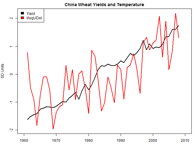
In 2011, I obtained the data for Lobell et al 2011 from lead author Lobell (who undertook at the time to place both data and code online, neither of which appears to be done.) I had asked Lobell to archive code, because it wasn’t entirely clear what he had done. Lobell collated temperature and precipitation data from both UDel and CRU. (For the latter, Lobell used the CRU TS data made famous by the Harry Readme.) In the figure below, I’ve plotted Lobell’s yield and temperature data for the China-wheat combination (both standardised to SD units), as an example of both series going up.
Lobell regressed Yield (actually log Yield) against time, temperature and precipitation variables, describing the procedure as follows:
Translating these climate trends into potential yield impacts required models of yield response. We used regression analysis of historical data to relate past yield outcomes to weather realizations. All of the resulting models include T and P, their squares, country-specific intercepts to account for spatial variations in crop management and soil quality, and country-specific time trends to account for yield growth due to technology gains (6).
The precipitation and quadratic terms don’t appear to affect the regression very much, i.e. the main effects are delivered by the model in which Yield is regressed against time and temperature as follows:
(1) Yield ~ Year + Temperature
Using conventional regression nomenclature, the regression coefficient b is given by the formula
(2) b= (X^T * X)^{-1} X^T y
where the X matrix of independent variables if {Year; Temperature} and y is the Yield vector.
For convenience (and thus is irrelevant to the point that I’m working towards), normalize the data.
X^T y is simply the vector of correlations of Yield to Time (the normalized trend) and Temperature.
(X^T * X) is nothing more than the correlation matrix between Year and Temperature i.e. the off-diagonal element r is the temperature trend (normalized units) as follows:
| 1 r |
| r 1 |
The calculation of the OLS regression coefficients uses the inverse of this matrix,
| 1 -r | * 1/(1-r^2)
| -r 1 |
The negative term in the off-diagonal means that the OLS coefficient for the regression of Yield onto Time and Temperature is calculated as a function of the correlation between yield and temperature, the trend in yield, the trend in temperature as follows:
b_temperature = 1/(1-r^2) (-r*trend_yield + cor_yield_temp)
In other words, if the correlation between Yield and temperature is less than the product of the trend in yields and trend in temperature (both normalized), then the regression coefficient is negative. This has nothing to do with yields or temperatures, but is a trivial property of the matrix algebra.
As an example, for the Chinese wheat series shown above, although there is a positive correlation between yield and temperature (0.5096), the OLS regression coefficient of a regression of Yield against Year and Temperature results in a negative coefficient. Applying the above formula, the normalized trends (correlations between year and item) for yield and temperature are 0.984 and 0.548, yielding 0.5096- 0.984*0.584 <0.


35 Comments
The main issue with this kind of statistical analysis is its short-term nature, whereby the “effect” of a variabñe is estimated by varying the said variable while keeping other variables constant. This ceteris paribus clause is not valid for long-term processes such as climate change.
Of course, given the use of a certain variety of a certain crop on a given field, under given agronomic practices, anysignificant deviation from “normal” temp and rainfall may cause a change, quite possibly a drop, in crop yields. But in the long term all variables change, and no ceteris is paribus any longer. Along five decades or a century, farmers will change te varietythey plant, and modify their farming practices, while soil properties are also likely to change. On an aggregate level (e.g. when entire countries are used as units of information) the zone where each crop is planted may vary, as well as the varieties used, and the country’s crop mix may change as well, in unforeseen ways. Keeping everything else constant makes no sense (its classic form is the Malthus fallacy of computing future corn production under an unchanging technology, as if the world would remain forever fixed in the conditions prevailing in 1798, when Reverend Thomas Malthus published his treatise on population.
Even a chain of short term OLS equations applied to all variables in successive years may also fail to capture the unexpected ways in which technology would change along the way. Recall the dire predictions of Lod Kelvin and others in the late 19th century, envisaging for instance London to be drowned under a mountain of horse manure by 1940 (no one expected horses to be replaced by cars, underground trains or even bikes, just as nobody foresaw mass aerial transportation).
Notice, by the way, that year-to-year changes in temp or rainfall are far greater than the respective secular trends foreseen by climate models (not to speak of the fact that “climate” is not the weather of each year, but an average computed over two or three decades); the equations, this fact notwithstanding, are based on year-to-year changes in temp and rainfall, “keeping the rest constant”.
Your math is correct. Another way of expressing the issue is to note that if the regression equation is Yield(t) = a + b1*Temperature(t) + b2*t + e(t), in other words if we regress Yield on Temperature + time, the coefficient on Temperature (b1) will be the same as if you regress detrended Yield on detrended Temperature. You could argue that there is an autonomous trend in Yield owing to technological improvements, so b2 is intended to capture it. But if that’s the model, you can’t then use the negative value of b1 to argue that future warming will be bad for agriculture, because by definition “the future” implies t goes up as well! In other words there is no logical way to construct a forecast in which Temperature goes up at some future point in time but t nevertheless stays constant.
They ought also to have added CO2 to the Yield model.
Thank you, Dr. McKitrick.
As someone whose command of statistics (and matrix algebra) falls woefully short of intuitive, I often find it challenging to navigate through Mr. McIntyre’s exposition; even working out a numerical example had in this case given me only a tenuous grasp of what the result really meant.
I always appreciate it greatly when you make his work accessible to us lesser lights.
+1 Joe!
+1, but its always interesting reading the explanations, simple and not.
Absolutely, Corey.
The only thing these data are tracking is the diminishing returns of the Green Revolution. What happens when they cherry pick the starting points.
RE: (notwithstanding the pause/hiatus in the 21st century)
I thought the pause/hiatus had been eliminated/cancelled, IE: it never happened. Tamino has graphs. Mann doesn’t remember publishing papers explaining how/why it happened before it didn’t happen. Trenberth said it was expected . . . but not until after it happened and then didn’t happen; which I’m guessing was also expected.
The U.S. and Canadian Government Agriculture Dept’s have all shown a steady rise in *all* crop yields. I’m thinking all major crop producing/exporting countries will have data showing the same steady increase. Apparently all due to new and improved farming practices and crop/plant engineering. And all in spite of climate change.
blob:https://ourworldindata.org/92f5bfdd-7152-48a0-8263-0fafddda6583
Crop yields mainly increasing since WWII, I don’t see any deterioration due to climate.
And what is the biological basis for assuming that small increases in average temperature have any effect on crop yield anyway? And what did they do about adjusting for growing season versus not, ripening requirements versus growing season, and all the other complexities of what is actually happening in terms of yield?
A “warmer” year might have all that extra warmth at the wrong time.
Not to mention that even if temperature has an effect on crop yields – and I think it likely does, that change would not have a consistent effect globally. Some locations would see improved yields, while other might lose. Also, the proposed temperature changes advanced by the AGW gang are to minor to have any significant effect.
Of course, the effect of warming may be moot. There was a recent BBC story about the people that raise the goats that produce true cashmere wool. These are seasonally transhumant nomadic people who graze their animals at very high altituds in the western Himalaya/Hindu Kush. They are having problems because the last few years snow has started about two months early and has been far too heavy for their animals to find grazing. They’ve relying on government support to keep their animals from starving. That early heavy snow puts the lie to any assertions about loss of ice or water shortages at least in the western portion of Southern Asia.
Amazing! The paper has 2471 citations.
I don’t know, perhaps this is all about the Law of Unintended Consequences. No one knows what will happen when the CO2 is doubled. It could be beneficial as in improved yield, but it also could all go horribly wrong. Even something like the improved yield goes along with the triggering of some competing pest that also thrives but destroys any benefits.
So getting the math wrong doesn’t really matter because no one can predict possible horrible outcomes — which is what being politically conservative is all about.
Thanos (hope you don’t mind me abbreviating your name), so far there is no evidence of harm in the nearly doubled C02 since the industrial revolution. Are “possible horrible outcomes” the only thing we should predict? I’m not confident in the prediction track record at this point anyway.
” No one knows what will happen when the CO2 is doubled. ” Greenhouse cultivators know. Submariners know.
Thanos
Can you explain to us with references what went “horribly wrong” in the Cambrian era, when multicellular life dramatically radiated and all phyla of living organisms alive today evolved? And when CO2 concentration in the air was 5000-20000ppm? Or what went “horribly wrong” during the 160 million years that the dinosaurs lived on earth while CO2 concentration in air was 1000-3000 ppm?
Or, to believe in CO2 warming alarm, is it necessary to believe that the world was created in 1850?
“…No one knows what will happen when the CO2 is doubled. …”
Thanos, there is a discipline called “Historic Geology.” Its subject is the entire geological history of the planet, including things like change in atmosphere. If you would be so good as to consult Geocarb III, then you would never have made such a glaringly wrong statement. roughly 150 million years ago, CO2 was at roughly 10 times “present” levels – that is 1950 CE. Around 250 million years ago, at the end of the Permian, right at the time of the largest extinction event we know, CO2 was at present levels. At about 550 million years ago CO2 was more than 20 times present levels. But, not only do we know what the consequences of “doubled CO2,” we also know the effects of low CO2. Currently we are seeing a “fertilizing” effect thanks to increased CO2 thanks to satellite imagery. More over, anyone genuinely interested in reality would do a bit of research and discover that lower CO2 levels than the present are troublesome and dropping below 180 ppm would quite possibly really trigger the sixth great extinction. Leave the echo chamber, look around, do some interdisciplinary reading, and quit taking cartoon characters seriously.
So another seminal climate paper has dodgy maths that should have been rejected by peer review and would shame any undergraduate if they submitted it. Yet the academic world will circle the wagons and support it. And they wonder why they are losing credibility.
Thank you SM for continuing to show that the foundations of the dogma aren’t even made of sand.
Indeed. Try to get into a discussion with any alarmist and they will claim Mann’s hockey stick is totally vindicated and “seminal science” as I just saw one state in a thread elsewhere. You could take all of the MBH 98 proxies, show them individually, that none but bristlecone pines have a hockey stick shape, and they will still blow you off. It’s amazing.
Papers with ‘some Maths’ need to be reviewed, or even coauthored, by Mathematicians with skills in the appropriate subset of Mathematics, not just those within the discipline of the paper.
As a Physics undergraduate, it was emphasised that our Maths lectures were being given by someone from the Department of Mathematics, not by our own department.
At the time, I thought what’s the difference?
The difference is that a Mathematician is an independent mind, focused on the Maths, with less chance of collusion, (we expect).
There are so many instances where this would have avoided a ‘mistake’, or even the paper from being written.
Steve
O/T In case you didn’t see Pointman on William Connelley
Start here, the Pointman link is included
A hearty congratulations to you and your partner Brian Murray for winning the 2020 US National over-70s squash doubles championship.
Oops.
Forgot to start congrats above with Steve’s name.
RE: ” . . . winning the 2020 US National over-70s squash doubles championship.”
Wow. Well done.
Staying upright for most of the day is considered a ‘win’ by me now . . .
Steve wrote: “the main effects are delivered by the model in which [log] Yield is regressed against time and temperature as follows”.
Unfortunately, I don’t fully understand much of what you and Ross wrote. On a decadal time scale, both temperature and time are highly correlated. Aren’t multiple linear regressions problematic when two explanatory variables are co-linear?
Since the mid-1970’s GMST has risen at an average rate of 0.19 +/- 0.03 K/decade (and was falling insignificantly before then). The same thing is true for temperature over land, except that the rate of rise is higher: 0.29 +/- 0.04 K/decade according to most indices (except GISS). Forcing has also been rising linearly (and significantly) since about 1975 (but not before). ASSUMING the temperature where wheat is being grown shows a similar pattern, I’d intuitively want to fit the following equations for the period since 1975:
T = a*t + e(t)
log(Yield(t)) = c*T + b*t = c*a*t + c*e(t) +b*t = (c*a+b)*t + c*e(t)
where a is the long-term rate of climate change, e(t) is “weather” (noise) in this long-term trend for year t, and b is the long-term rate of improvement in yield due to technological improvements. If we regress the log of the detrended yield vs detrended temperature = weather = e(t), we can determine c, the effect of temperature on yield:
detrended temperature = e(t)
detrended log(yield) = c*e(t)
trend in temperature = a*t
trend in log(yield) = c*a + b
Once we know c and a, then we can determine b, the rate of technological improvement. And I want to know the confidence intervals for these values, not merely their central estimates.
Now that I’ve worked through all of these steps, they sound similar (but perhaps not identical) to what both you and Ross wrote. If this amateur approach makes any sense, perhaps your readers would appreciate seeing the relevant plots.
(I cherry-pick 1975 as a starting point because I know that long-term trends in forcing and warming are significantly large and linear after, but not before, this “inflection point”. However, since you often disapprove of any form of cherry-picking, there is no reason one couldn’t use all of the data since 1960, which would likely include a run of cold “weather” – negative e(t) terms – before significant forced global climate change began after about 1975.)
Michael Mann’s letter to the editor in today’s Boston Globe (3-19-20)
“I am relieved to see policy makers treating the coronavirus threat with the urgency it deserves. They need to do the same when it comes to an even greater underlying threat: human-caused climate change.
In a recent column (“I’m skeptical about climate alarmism, but I take coronavirus fears seriously,” Ideas, March 15), Jeff Jacoby sought to reconcile his longstanding rejection of the wisdom of scientific expertise when it comes to climate with his embrace of such expertise when it comes to the coronavirus.
In so doing, Jacoby took my words out of context, mischaracterizing my criticisms of those who overstate the climate threat “in a way that presents the problem as unsolvable, and feeds a sense of doom, inevitability, and hopelessness.”
As I have pointed out in past commentaries, the truth is bad enough when it comes to the devastating impacts of climate change, which include unprecedented floods, heat waves, drought, and wildfires that are now unfolding around the world, including the United States and Australia, where I am on sabbatical.
The evidence is clear that climate change is a serious challenge we must tackle now. There’s no need to exaggerate it, particularly when it feeds a paralyzing narrative of doom and hopelessness.
There is still time to avoid the worst outcomes, if we act boldly now, not out of fear, but out of confidence that the future is still largely in our hands. That sentiment hardly supports Jacoby’s narrative of climate change as an overblown problem or one that lacks urgency.
While we have only days to flatten the curve of the coronavirus, we’ve had years to flatten the curve of CO2 emissions. Unfortunately, thanks in part to people like Jacoby, we’re still currently on the climate pandemic path.
Michael E. Mann
State College, Pa.
The writer is a professor at Penn State University, where he is director of the Earth System Science Center.”
So, Mann descends to the level of Greta with emotive statements like “the truth is bad enough when it comes to the devastating impacts of climate change, which include unprecedented floods, heat waves, drought, and wildfires that are now unfolding around the world” while at the same time appealing to “the wisdom of scientific expertise when it comes to climate”? Enough said.
That’s amazingly pathetic, even by Mann’s standards.
At the very minimum, it’s “tone-deaf.”
Maybe I’m wrong, but given the inaccuracy of early coronavirus modelling, it seems only reasonable that climate models should be viewed with greater uncertainty.
The coronavirus models were based on timescales of just a few days, a few weeks or at most two months. These models have demonstrated the limitations of modeling, or maybe more accurately the limitations of modelers to develop reliable models.
George,
There is a peer reviewed article that will appear in the journal “Dynamics of Atmospheres and Oceans” that proves that global climate and weather models are based on the wrong dynamical system of equations. Thus any conclusions based on those models are not reliable (to say the least).
I hvae earlier provided an example on this site that shows that if one is allowed to choose the forcing in any time dependent system, even if it has nothing to do with reality, one can produce any solution one wants. In particular one can reproduce historical data with the wrong model.
Jerry
Steve,
Can you audit Ferguson et al (2019), which is influencing UK govt policy?
Click to access Imperial-College-COVID19-NPI-modelling-16-03-2020.pdf
Potential problems include a too-high case fatality rate and assumption of constant critical care capacity rather than a capacity that scales up fairly rapidly.
Ferguson recently acknowledged: “I’m conscious that lots of people would like to see and run the pandemic simulation code we are using to model control measures against COVID-19. To explain the background – I wrote the code (thousands of lines of undocumented C) 13+ years ago to model flu pandemics…”
Stephen, this does not belong here, but I do not know any other way to contact you
COVID19 Effect on CO2 levels
An analysis of recent CO2 levels in the light of drastic reductions in industrial activity. Guess what? CO2 did not go down!
Ray, there was also a large decrease in the amount of fossil fuels used during the great depression, but no measured decrease nor deceleration in CO2 concentration from the Ice cores drilled at Antarctica.
I can provide the data for anyone who is interested.
Off-topic – sorry:
foia.org appears to have been hacked or possible lapsed and taken over by a (Chinese?) website about epilepsy.
And then of course, there is the matter of the carefully selected (?) time-frame (1961 – 2008). The 1960s were one of the coolest periods in the last century.
If the time period had extended back to (say) the 1930s, I suspect the findings would have been completely different.
3 Trackbacks
[…] https://climateaudit.org/2020/03/02/ipcc-ar5-wg2-on-yield-sensitivity-statistical-malpractice/ […]
[…] IPCC AR5 WG2 on Yield Sensitivity: Statistical Malpractice […]
[…] https://climateaudit.org/2020/03/02/ipcc-ar5-wg2-on-yield-sensitivity-statistical-malpractice/ […]