Climate Audit

Nearly all of the text of this article on an interesting ice core proxy series (James Ross Island) from the Antarctic Peninsula was written in June 2014, but not finished at the time for reasons that I don’t recall.  This proxy was one of 16 proxy series in the Kaufman 12K pdf. 60-90S reconstruction.

I originally drafted the article because it seemed to me that the then new James Ross Island isotope series exemplified many features of a “good” proxy according to ex ante criteria that I had loosely formulated from time to time in critiquing “bad” proxies, but never really codified (in large part, because it’s not easy to codify criteria except through handling data.)

Although this series is in the Kaufman 60-90S reconstruction, its appearance is quite different than the final 60-90S reconstruction: indeed, it has a very negative correlation (-0.61) to Kaufman’s final CPS reconstruction. I’ll discuss that in a different article.

Following is mostly 2014 notes, with some minot updating for context.

“Good” Proxies
I’ve articulated with increasing clarity over the years (but present in early work as well) – is that one needs to work outward from proxies that are “good” according to some ex ante criteria, rather than place hope in a complicated multivariate algorithm on inconsistent and noisy data, not all of which are “proxies” for the item being reconstructed. This is based on principles that I’ve observed in use by geophysicists and geologists to combine “good” (high resolution) data with lower quality data.

While I haven’t attempted to reduce my concepts of a “good” proxy, over the years, I have developed some criteria that I find useful in appraising proposed proxies. I will briefly assess the James Ross Island isotope series against these criteria.

First, for a class of proxy to be useful in a reconsruction network, it ought to have been applied to many locations, rather than being an ad hoc singleton. For example, one of the few PAGES2K (South America) reaching to medieval period was an index from Lago Aculeo pigments. This was a novel and then unique proxy class.  Even if pigment proxies ultimately prove to be ideal, there was only one example available to PAGES2K. Without many examples, we simply don’t know how it might be confounded. In contrast, there are dozens of polar ice core isotope series, qualifying this proxy class on this count.

Second, a good proxy needs to be both high resolution and well-dated. Ice cores are dated with high accuracy. (Ocean sediments are not as well dated). “High” resolution depends on the context: I much prefer proxies that have at least 10-year resolution. The resolution of the James Ross ice core deteriorates with age, but it performs well on these counts as compared to (say) most ocean sediments.

Third, I place particular value on high-resolution proxies that extend through the Holocene. The changes from the LGM to the mid-Holocene to the present are sufficiently great that one can benchmark which way is up for the proxy class. It sounds obvious, but I think that it’s more important than generally acknowledged. Antarctic (and Greenland) ice cores are a very important example of such proxies.

Fourth, for Holocene-scale reconstructions, one needs proxies that are responsive to millennial scale changes.  Esper et al 2012, an excellent article, observed that very long tree ring chronologies extending back to the Mid-Holocene (a few Scandinavian series) lacked the millennial-scale variation that “ought” to be observable given the dramatic changes in NH high-latitude summer insolation over this period (which is much, much greater in comparison to CO2 forcing than most people would expect.)  In the Arctic, there is evidence that “small” ice caps may provide more nuanced information on Holocene changes than the Greenland summit. Gifford Miller’s work on Baffin Island is one example (covered in several CA posts http://www.climateaudit.org/tag/miller); there is also interesting work on proglacial lakes adjacent to small Greenland ice caps (Bregne, Istorvet, Renland) which show mid-Holocene warmth more clearly than ice core proxies from the summit of the main Greenland ice sheet.

Fifth, one needs proxies that are relatively free of secular drift which distorts the relationship between the proxy and temperature. In ice cores, this can happen in several ways. For example, because glaciers flow, the source ice from deeper sections of an ice core can come from higher elevations, imparting an extreme bias to the series. Masson (2000) contained some striking examples. The earliest Agassiz cores (1977; 1979) also had this problem (but were uncritically used in some multiproxy articles nonetheless.)  Specialists attempt to mitigate this problem through locating cores at summits, but these attempts are not always successful. Ice core series which suffer from this problem ought not to be used (though they sometimes are).

Sixth, for ice core proxies, changes in elevation of the Greenland and Antarctic ice sheets through the Holocene (mostly lowering) result in an important long-term drift in the association between isotopes (d18O, d2H) and temperature. Vinther (2009) proposed (in my opinion) a really elegant solution to this problem: he noticed that elevation changes over the Holocene in adjacent small ice caps (Agassiz on Ellesmere Island, Renland in east Greenland) were MUCH less than at the top of the Greenland ice sheet.  The isotope series from these small ice caps had a close relationship with the more famous series from the top of the Greenland ice sheet (GISP, GRIP), but there was a noticeable increasing difference in levels between the series over the long Holocene.  Vinther plausibly attributed the long-term change to elevation decrease of the Greenland ice sheet through the mostly warm Holocene and used the difference to estimate the elevation change. Vinther also observed that the decreasing isotope trend in Renland and Agassiz series was very coherent with the decline in summer NH insolation (the driving force in Milankowitch theory), while the GISP2 series (hugely popular with “skeptics”) was very flat, too flat.  Under Vinther’s analysis, after allowing for elevation change, the GISP2 series is no longer flat, but declining through the Holocene, just like the Renland and Agassiz series.

While the authors of the James Ross Island dataset didn’t connect their site location to Vinther’s conceptual model, James Ross Island,  which is separate from the Antarctic Ice Sheet and very small in comparison, also has the key features of the Renland and Agassiz series that Vinther used for his benchmark, thereby offering the possibility of a similar benchmark for series from locations on the Antarctic ice sheet where large changes in elevation are known to have occurred e.g. Law Dome.

It is the first ice ice core from the Antarctic Peninsula which extends to the start of the Holocene and earlier.  There have been several previous ice cores on the Peninsula, but none even reached 1500 years. The nearest ice cores reaching into the Holocene and LGM are approximately 60 degrees away each in both directions: Dronning Maud at 3E and the new WAIS core at 112W, both much further to the south on the Antarctic continent.

This is not to say that the James Ross Island isotope series will not prove to have warts of its own, but it has many features that it make it more interesting ex ante than yet another ex post screened tree ring chronology.

In passing, I find speleothem isotope series, though mostly given little attention in multiproxy articles, to be very interesting proxies, as they are (1) highly replicated: (2) consistent between nearby sites; (3) well-dated; (4) both reach back through the Holocene to the LGM and come forward to the very present.  Chinese data appears particularly thorough.

The James Ross Island dD Series
The James Ross Island isotope series was originally published as Mulvaney et al (Nature 2012), Recent Antarctic Peninsula warming relative to Holocene climate and ice-shelf history pdf.  Another publication by the same authors (^) is limited to the period from AD1000 on, which is highlighted in light yellow below.

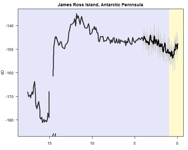Figure 1. James Ross Island dD, showing post-1000 AD values in light yellow margin. The LGM ice (separation denoted by //) is NOT dated 

The main features of the James Ross Island data are obvious.

The LGM (not dated here) is very cold. The highest values of the series are in the Early Holocene (12.5-10 ka BP). Values from ~9000 BP to 3000 BP fluctuated within a relatively narrow range before declining in the late Holocene (after ~4000 BP). The lowest values were reached about 500 BP, more or less contemporary with the NH Little Ice Age. Values in the 20th century were higher than in the LIA, but are still lower than values through most of the Holocene an considerably lower than the highs in the Early Holocene.

Notwithstanding its rather deceptive title (Recent Antarctic Peninsula warming relative to Holocene climate and ice-shelf history), Mulvaney et al recognized these features in an extended and interesting discussion of the data, including the following (and other similar comments):

The Holocene temperature history from the JRI ice core is characterized by an early-Holocene climatic optimum that was 1.3 +- 0.3 deg C warmer than present (Fig. 3). The magnitude and progression of this early-Holocene optimum is similar to that observed in ice-core records from the main Antarctic continent [16 –Masson-Delmotte 2011]…

Likewise, marine temperatures on the western side of the Antarctic Peninsula [17-Shevenell 2011] declined to reach, by ~8,000 yr BP, a long-term mean that was close to present-day values…

Various proxy evidence exists for a mid-Holocene warm period on the Antarctic Peninsula [7- Bentley 2009], although the lack of a consensus on its timing in this region may be explained by the small magnitude of this feature in the JRI temperature record compared with the well defined mid-Holocene climate optimum in continental Antarctic icecore records [16 – Masson Delmotte]…

Marine sediments indicate that a permanent ice shelf was established there [Prince Gustav] only after ~1,500 yr BP and that the maximum ice-shelf extent may have been reached as recently as a few centuries ago [3 –Pudsey 2006].

Despite these sensible comments, the abstract to Mulvaney et al 2012. in apparent genuflection to the “consensus”, began with the words “rapid warming over the past 50 years” and observed that “the high rate of warming over the past century is unusual (but not unprecedented) in the context of natural climate variability over the past two millennia”.

Conclusion

To the extent that proxies and proxy reconstructions have broader significance in the climate debate, their interest largely arises from the unprecedentedness (or lack thereof) of late 20th century/early 21st century data relative to the past.  When IPCC was founded, as much interest attached to the comparison of the modern warm period to the “Holocene Optimum” (or “Holocene Thermal Maximum”) as to the corresponding comparison to the medieval warm period.  In the 1990s and, especially since the IPCC Third Assessment (2001) promoted the Mann hockey stick, far more attention has been paid to the medieval comparison, but there is increasing interest in the longer Holocene perspect (Marcott et al 2013; Kaufman 12K (2020).