CRU Responds

CRU has posted up an undated webpage on data availability here , responding to the various recent FOI requests for station data and confidentiality agreements. Here they “list the agreements that we still hold”.

I’m preparing a post on this extraordinary document and am posting this thread as a placeholder for now.

Instalment 1 (Aug 11 8 pm) :
Obviously this is a pretty pathetic combination of excuses and whining. Both CRU and the Met Office should be cringing with embarrassment. Obviously there will be more shoes to drop. But let me reiterate one of my own baseline positions (and one which I do not wish to argue about with readers.) Regardless of how pitiful CRU’s management of data and contracts turns out to be, it is not my position that this is an excuse for delaying climate policy until the original data is found and documented. Neither do I think that any exigencies of the big picture excuse negligence in the small picture.

Lost Data
Surely the most surprising revelation is their confession that they’ve lost all their original data – all they have is their “value added version”. They say:

Since the 1980s, we have merged the data we have received into existing series or begun new ones, so it is impossible to say if all stations within a particular country or if all of an individual record should be freely available. Data storage availability in the 1980s meant that we were not able to keep the multiple sources for some sites, only the station series after adjustment for homogeneity issues. We, therefore, do not hold the original raw data but only the value-added (i.e. quality controlled and homogenized) data.

I was around in the 1980s and the 1970s. People used filing cabinets back then. You’d have alphabetically arranged files by customer. If you got paper from Andorra or Zambia, you’d put the data in the Andorra or Zambia file. If a decision were made on the handling of an account, you’d put a memo in the file. How is it possible that they don’t have ANY documentation on the construction of their data? This is getting worse and worse.

CRU Excuses
Imagine [you fill in the name] saying something like this:

Below we list the agreements that we still hold. We know that there were others, but cannot locate them, possibly as we’ve moved offices several times during the 1980s.

Nobody would take it seriously. Nobody would believe that they were that incompetent. I wonder what would happen if Lonnie Thompson moved offices. Would he lose all his unarchived ice core data?

Or this excuse as to why they can’t get data that any one of us can locate on the internet:

Much climate data are now additionally available through the internet from NMSs, but these are often difficult to use as data series often refer to national numbering systems, which must be related back to WMO Station Identifiers.

Poor babies. Imagine having to do a concordance of CRU numbers to national numbers to enable downloading from NMSs. That would be so boring. After all, they’re climate scientists. Things to do, people to see. When’s the next IPCC authors’ workshop?

But their trials and tribulations get even worse. They report that:

a number of NMSs make homogenized data … available in delayed mode over the internet. Some that provide both raw and homogenized versions, generally do not link the two sets of data together.

Y’mean, that someone somewhere would actually have to inquire as to how to do the links. Hey, Phil, I’ve got an idea. If they won’t tell you, send them an FOI. Or better yet, we’ll save you some trouble. Make a list of all the NMSs that are troubling you and we’ll send FOIs for you. Just have your people contact our people.

And as to why they haven’t documented the source of their data. It’s not their fault – that’s impossible. The reason why they didn’t document anything is that they “never had sufficient resources”.

We are not in a position to supply data for a particular country not covered by the example agreements referred to earlier, as we have never had sufficient resources to keep track of the exact source of each individual monthly value.

Some Data and Scripts for BS09

The controversy between Benestad and Schmidt on the one hand and Scafetta and West on the other hand is a typical climate science dispute, in that neither of the parties has provided scripts evidencing their analysis. [Note: BS09 provides url’s for data versions used; SW do not.]

Scafetta and West provide a plausible criticism of BS09 – that they used cyclic padding in their wavelet analysis – but Schmidt says that this doesn’t “matter”. Perhaps it does, perhaps it doesn’t. The Team never admits that errors “matter” (even when they do) so third parties may be forgiven for taking Schmidt’s recent claim of not mattering with a grain of salt.

In order to arrive at an informed opinion – as opposed to be swayed by the rhetoric on either side – one has to look at the data and carry out wavelet analysis as described by the authors. Most people aren’t interested enough in the dispute to try to figure out what they did and thus will simply agree with the rhetoric of the side that they prefer.

I requested scripts from both Schmidt and Scafetta without success. Schmidt did not respond to my email. Scafetta replied but was busy on other matters for a while.

As it happens, the wavelet package used in BS09 was the same package (waveslim) as we used in our treering simulations in MM2005(GRL). Indeed, Schmidt used the same wavelet (“la8”) as we used. I’ve downloaded solar data in the past. So, in the absence of scripts from either party of climate scientists, I thought that I might be able to get a foothold on the data fairly quickly. It turned out not to be quite as quick as I planned, but I’ve made my foothold available here for others who may be interested in the dispute.

To simplify access to these materials, I’ve placed some tools online (www.climateaudit.org/scripts/solar) and have carried out my own wavelet analysis, obtaining a result that appears intermediate between Schmidt and Scafetta. It turns out that there is a pretty obvious obvious criticism of the Scafetta analysis that Schmidt didn’t make – perhaps because we criticized them for this in Santer et al 2008.

First, here is the original Scafetta wavelet smooth of the solar data. Their data set is a splice of Lean 1995 and ACRIM, with an offset to Lean in 1980 to splice the two data sets.

The period 1900–1980 is covered by the TSI proxy reconstruction by Lean et al. [1995] that has been adjusted by means of a vertical shift to match the two TSI satellite composites in the year 1980.


Figure 1. From Scafetta and West 2006.

Here’s a script to get ACRIM, PMOD and Lean data and then splice them according to the procedure of Scafetta and West [Upate: (GRL March 2006) procedure here; the procedure of Scafetta and West (GRL 2007) is a little different centering on 1980-1991)]

#Get Solar Data (making Acrim and pmod into monthly series)
source(“http://data.climateaudit.org/scripts/solar/collation.functions.solar.txt”)
pmod=get.solar(dset=”pmod”)
acrim=get.solar(dset=”acrim”)
lean=get.solar(dset=”lean95″);tsp(lean) #1600 1999

#Make annual averages of monthly information
acrim.annual= annavg(acrim)
pmod.annual= annavg(pmod)

#Do splice a la Scafetta-West 2006
Solar=ts.union(window(lean,start=1817),acrim.annual,pmod.annual)
Solar=data.frame(year=time(Solar),Solar)
names(Solar)=c(“year”,”lean”,”acrim”,”pmod”)
(delta.acrim= Solar$acrim[1980-1816]-Solar$lean[1980-1816]) # -1.476112
(delta.pmod= Solar$pmod[1980-1816]-Solar$lean[1980-1816]) # -1.476112
#SW centers on 1980 a la SW06, slightly different centering in SW07
temp= Solar$year>=1980
Solar$acrim.splice=Solar$lean+delta.acrim
Solar$acrim.splice[temp]=Solar$acrim[temp]
Solar$pmod.splice=Solar$lean+delta.pmod
Solar$pmod.splice[temp]=Solar$pmod[temp]

Next here is an updated function that extracts the wavelet decomposition using reflection at the boundary, instead of default periodic. [Aug 10: This use of the option within mra replaces an awkward patch in yesterday’s version in which I inserted a long reflection pad, used the default on the padded version and truncated back. The old script is retained in the scripts directory for people desperate to see an awkward programming decision.]

#this pads the series by reflection
wavelet.decomposition< -function(x,wf0="la8") {
N<-length(x)
#steps to interpolate missing data not relevant here
y=x
temp<-!is.na(y)
ybar<-mean(y,na.rm=TRUE)
y<-y[temp]-ybar
N1<-length(y)
J0<-trunc(log(N1,2))
mod.y<-mra(y,wf0,J0,"modwt",boundary="reflection")
names(mod.y) #[1] "D1" "D2" "D3" "D4" "D5" "D6" "D7" "D8" "S8"
test<-mod.y[[1]]
for (i in 2:(J0+1)) test<-cbind(test,mod.y[[i]])
dimnames(test)[[2]]=names(mod.y)
return(test)
}

Now we’ll do a wavelet decomposition with padding and plot the results.

temp=(1881:2008)-Solar$year[1]+1
model=wavelet.decomposition(Solar$acrim.splice[temp] ,wf0=”la8″)
(ybar=mean(Solar$acrim.splice[temp] ) )# 1365.152
dim(model) #[1] 256 8
decomp=cbind(R2=apply(model[,c(“D1″,”D2″)],1,sum), D3=model[,”D3″],D4=model[,”D4″],S4=apply(model[,5:ncol(model)],1,sum) )
par(mar=c(3,4,2,1))
plot(1881:2008, Solar$acrim.splice[temp],type=”l”, ylab=”Irradiance (wm-2)”)
title(“ACRIM Irradiance”)
lines(1881:2008,decomp[,”S4″]+ybar,col=2)
mtext(side=1,”ACRIM Spliced with Lean 1995 per Scafetta-West 2006″,cex=.7,line=1.7)

This yields the following graphic.

Figure 2. Emulation of SW06 using up-to-date data

As you can see, the wavelet smooth dips down towards the end (whereas the corresponding smooth in SW06 doesn’t) but not quite as much as BS09.

The explanation is interesting as the probable reason why Schmidt didn’t comment on it.

I’ve marked the year 2000 with a dotted line here. Whereas Santer (Schmidt) et al 2008 used data ending in 1999, Scafetta West’s diagram ends in 2000, although solar data is obviously available since then. [Lucia emailed me that the Scafetta data ends in 2002 – the point is still the same.]

Making a S4 smooth with padded values based on a 2000 (or 2002) endpoint creates an uptick, whereas using actual values through to 2008 yields a downtick. Perhaps not as big a downtick as cyclic reflection. However, the downturn since 2000 (or 2002) has been substantial enough to substantially mitigate the error introduced by the incorrect cyclic padding procedure. So some of Scafetta’s victory here may be a bit rhetorical as the error may actually not “matter” as much as much as one would have thought. [

Note that Rahmstorf’s linear padding or Mannian padding would have resulted in the same sort of problem. This is actually a pretty interesting example of padding impact. I’ve criticized the use of these sorts of smoothed series in regression analyses elsewhere. I haven’t waded further through the articles to see what exactly they did downstream of this point, but, if they used smoothed series in regression analysis, what’s sauce for the goose is sauce for the gander.

The Dog That Didn’t Bark
Note that it was open to Schmidt to observe that Scafetta-West had used an obsolete data set ending in 2000 (or 2002), but they didn’t do so. Why?

My guess is that we recently criticized Santer (Schmidt) et al 2008 in a comment submitted to IJC for exactly the same thing – using obsolete data ending in 1999. Obviously if Gavin argued the point here, it would be used against him in reviving our comment on Santer et al 2008. So instead, he preferred to apply an incorrect procedure. But hey, it’s climate science.

UPDATE Aug 10: There’s an easy of doing a boundary reflection in the mra algorithm: specify boundary=”reflection”. In yesterday’s script, I added a long reflection pad while still using the default (an awkward patch reminiscent of Mann’s butterworth padding). This patched the problem but using the right option is easier and has implemented been inserted in the above code. Here’s the difference between the results with an endpoint in 2002 (which I believe was used in SW06) and an endpoint in 2008. Nicola Scafetta has written in comments below that reflection in 2002 is “right” and reflection in 2008 is an “error”. I haven’t reflected on these comments yet and, at this stage, merely show the difference. For comparison, I’ve also shown the effect of Rahmstorf smoothing based on a 2002 endpoint.

Figure 3. Showing impact of different end points and Rahm-smoothing.

NOAA: HadCRU3 data not "influential"

A CA reader recently wrote to NOAA (which distributes HADCRU3 gridded data) asking them whether the data and methods had been reviewed pursuant to NOAA Quality of Information guidelines. (It is nice to see a reader complete such an exercise himself rather than writing on a thread that I should do it.) NOAA replied that they had not done so because the data came from a third party and that HADCRU3 data “do not meet the definition of influential”. One wonders what sort of data NOAA regards as “influential”. Here’s the correspondence:

The CA reader wrote:

I believe that the HADCRU3 dataset is influential scientific information, which although generated by a 3rd party, is of such importance that it is important that it be of known quality and consistent with NOOA’s information quality guidelines.

Has NOAA reviewed the raw data and processing methods in accordance with NOAA’s Quality of Information standards?

Does NOAA have available the raw station data and metadata and processing algorithms behind the HADCRU3 gridded data? If so, I request a copy of such data, metadata, and processing information.

I would also like to know the nature and description of any specific checks used by NOAA to ensure the objectivity of the HADCRU3 dataset.

Best Regards,

Reader

NOAA replied:

Dear …:

Thank you for your inquiry regarding the HADCRUT3 gridded data available on the National Oceanic and Atmospheric Administration’s (NOAA) Office of Oceanic and Atmospheric Research (OAR) website: http://www.cdc.noaa.gov.

NOAA OAR’s Climate Diagnostics Center is now part of the Earth System Research Laboratory, Physical Sciences Division (ESRL/PSD). ESRL/PSD makes available many climatological and meteorological datasets, as a service to the research community and to the general public. ESRL/PSD is not the originator of these datasets.

In the case of the datasets in question, the originator is the United Kingdom’s Meteorological Office’s Hadley Centre for Climate Change. Please refer to the page you reference in your inquiry and you will note the Hadley Centre is identified as the “original source”. Links to the Hadley Centre are also offered on the ESRL/PSD web page: http://hadobs.metoffice.com/hadcrut3/

The HADCRUT3 datasets are third party information. NOAA’s policies regarding dissemination of third party information are specified in the NOAA Information Quality Guidelines:
http://www.cio.noaa.gov/Policy_Programs/IQ_Guidelines_110606.html, as well as the OMB Peer Review Bulletin. According to NOAA IQ Guidelines, when the agency disseminates information supplied by a third party, the agency should review the OMB Peer Review Bulletin for applicability. According to the provisions of the OMB Peer Review Bulletin, dissemination of an information product is not covered unless it represents an official view of the agency. The Hadley Centre datasets do not represent an official view of NOAA. Further, even if the datasets did contain an official agency view, the peer review requirements would apply only if the dissemination of information is “influential”; which is defined to mean, “the information will have or does have a clear and substantial impact on important public policies or private sector decisions”. NOAA OAR has determined that the Hadley Centre datasets do not meet the definition of influential since the data will not have a clear and substantial impact on important public policies or private sector decisions.

ESRL/PSD makes every effort to ensure that the informational content of HADCRUT3 datasets available on NOAA/OAR’s website are the same as the original data disseminated by the Hadley Center. The NOAA IQ Guidelines provide that the accuracy of original and supporting data within an acceptable degree of imprecision or error, are by definition within the agency standard, and therefore presumed to be considered accurate. Because the HADCRUT3 datasets constitute original data, this standard applies and the datasets are presumed to be accurate under the NOAA IQ Guidelines.

As a re-disseminator, and not the originator of the data, ESRL/PSD does not maintain raw station data, nor is ESRL/PSD the correct source for information regarding the processing algorithms used to create the datasets. That information can be found on the Hadley’s Centre’s website and also in the published literature, referenced and/or linked on the web page.

Thank you, and good luck with your inquiries.

Sincerely,

Nick Wilde

Dr. Nick Wilde, Senior IT Manager,
Physical Sciences Division, Earth System Research Laboratory

Rahmstorf Sea Level Source Code and Transliteration

There has been considerable recent blog discussion of Rahmstorf smoothing and centering, with attention gradually being increasingly directed towards Rahm-sea level.

Last year, these topics were discussed online by Tom Moriarty here in a posting at his blog which unfortunately did not receive as much attention as it deserved. Following recent discussion at CA, Tom posted a follow-up article here. Tom and I got in touch and, from that correspondence, I learned that Rahmstorf had commendably sent code for his sea level article to Tom, commenting that he was “the first outside person to test this code”.

As we’ve learned, such testing is not a prerequisite for publication in the most eminent science journals (Science in this case) nor for use in “important” reviews, such as the Copenhagen Synthesis.

I’ve placed the (Matlab) code online here. I’ve transliterated some relevant portions and placed source data online so that the emulation is turnkey.

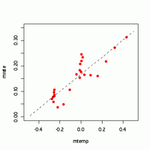
I’ll demonstrate that I’ve got the right data and have emulated things correctly. I’ll conclude this post with an interesting plot of the actual data – something that was omitted in Rahmstorf 2007.

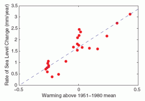
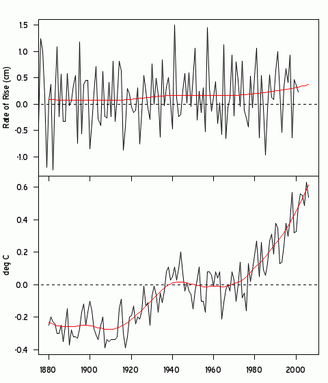
Ramhstorf first rahm-smooths the GISS temperature and sea level ( as usual, using ssatrend Rahmstorf “15-dimensional embedding”, which I’ve shown elsewhere to be an alter ego for a 29-point triangular filter). Then he calculated the sea level rise. Then he binned both into 5-year intervals and did (in effect) a linear regression. R07:

A highly significant correlation of global temperature and the rate of sea-level rise is found (r = 0.88, P = 1.6 × 10⁻⁸) (Fig. 2) with a slope of a = 3.4 mm/year per °C.

These results are obtained through a simple linear regression of binned and smoothed rise against binned and smoothed temperature. No allowance is made for the reduced degrees of freedom for autocorrelation. (After making such an allowance, needless to say, there are virtually no degrees of freedom left.) R07 illustrated this regression through his Figure 2, emulated below. This “relationship” is used throughout the article.

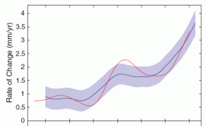
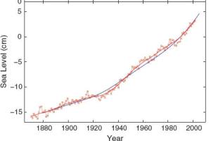
Next here is an emulation of the top panel of R07 Figure 3, showing the smoothed rate of sea level rise against the fit from the smoothed GISS temperatures. (Actually and this is something that may surprise readers – the red curve has been rahm-smoothed twice!) I’ll show some further information on this “relationship” below.

Figure 2. Emulation of R07 Figure 3 top panel.

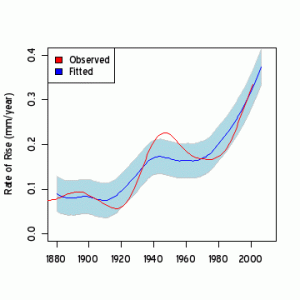
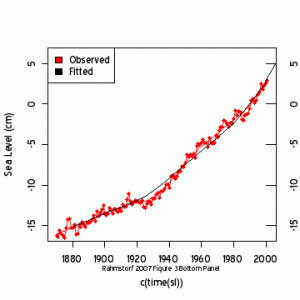
Next here is an emulation of R07 Figure 3 bottom panel, showing the fit of the semi-empirical relationship – this is carried forward into the Figure 4 projections which follow/

Figure 3. Emulation of R07 Figure 3 bottom panel.

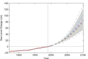
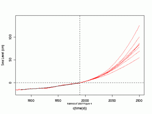
Rahmstorf then takes various IPCC projections and uses the R07 “relationship” between temperature and sea level to project sea level.

Figure 4. Emulation of R07 Figure 4.

Something that isn’t actually shown is R07 is a plot of the data, an omission which is remedied below. To me, these curves look like they have very little relationship. But if you’re a Copenhagen Synthesizer or a Science reader, this relationship is, I guess, 99.99999% significant.

What happens when the Rahmstorf relationship is adjusted for autocorrelation, along the lines of the Steig corrigendum (or the Santer, Schmidt 2008 critique of Douglass et al 2007).

There are only 24 bins. The AR1 autocorrelation of residuals is 0.75, resulting in N_eff of 3,36 (using N_eff=N*(1-r)/(1+r) ).

Whereas the OLS standard error was 0.039, the AR1 adjusted standard error is 0.156 (using:

se.obs= sqrt((N-2)/(neff-2))* summary(fm)$coef[2,”Std. Error”];se.obs

With the reduced degrees of freedom, the benchmark t-statistic is closer to 3 than to 2:

t0= qt(.975,neff) # 2.997517

Instead of a rahm-significant relationship as claimed, the confidence intervals are: 0.34 \pm 0.47 (not significant at all).

(ci=t0*se.obs) # 0.4659963

Having said that, it makes sense to me that higher temperatures would result in higher sea levels. I think that a heuristic diagram comparing the total sea level rise to the total increase in temperature in the historical period would probably make some sense. It’s Rahmstorf’s effort to dress a heuristic relationship in the language of statistics that fails so miserably. With the recent Steig precedent on the need to issue a corrigendum for failing to allow for autocorrelation, Rahmstorf really needs to do a similar corrigendum.

It’s pretty hard to keep up with Team corrigenda.

BS09 and Mannian Smoothing

Many CA readers have probably noticed Lucia’s recent coverage of Benestad Schmidt (JGR 2009) (with the inevitable acronym BS09). BS09 was an effort by B&S to verify Scafetta and West.

realclimatescientists can also be climateauditors, I guess. It’s too bad that they don’t spend the same amount of energy examining Mann et al 2008 or something like that.

Scafetta replied to BS09 at Pielke Sr here. The rebuttal point that interested Lucia was an issue relating to end points. Scafetta argued that BS09 had failed to understand wavelet decomposition and urged the BS authors to study a wavelet primer. While I’ve used wavelet decomposition in R from time to time and have written algorithms using modwt, my initial reaction was that once they started arguing about wavelets, you’d have to see their scripts to fully understand what the dispute was about.

In fact, the matter is much simpler than that and pertains only to end-point padding, an issue that we’ve covered here on a number of occasions, especially in connection with Mannian smoothing and Rahmstorf smoothing. Lucia referred to the latter discussion, but the discussion has been going longer than that.

As we’ve discussed, there are several methods in play for endpoint padding to create a smooth: padding with the mean (IPCC); reflection; reflection-and-flipping (Mann); linear extrapolation (Rahmstorf).

An option embedded in some algorithms – one which is highly inappropriate for trending series – is “cyclic” padding. Where you pad the end with values from the beginning.

Here is BS09 Figure 4. Note in particular the downslope of the smoothed version of the various series at the end.

Figure 1. Excerpt from BS09.

In his rebuttal at Pielke Sr, Scafetta observes that the BS09 smooth was derived by cyclic padding. . Scafetta observed:

By applying a cyclical periodic mode Benestad and Schmidt are artificially introducing two large and opposite discontinuities in the records in 1900 and 2000, as the above figure shows in 2000. These large and artificial discontinuities at the two extremes of the time sequence disrupt completely the decomposition and force the algorithm to produce very large cycles in proximity of the two borders, as it is clear in their figure 4. This severe error is responsible for the fact that Benestad and Schmidt find unrealistic values for Z22y and Z11y that significantly differ from ours by a factor of three

Here is the figure illustrating the point:

Figure 2. Figure from Pielke Sr blog illustrating the cyclic padding in BS09.

This particular issue is unrelated to wavelet decomposition in the sense that cyclic padding with a gaussian filter or something like that would have yielded a more or less similar smooth. In the latter case, however, you’d have had to make a decision on endpoint padding and even the BS09 authors would have been unlikely to include cyclic padding in their written description. It seems to have crept in as a default mechanism in the algorithm, to the authors’ bad luck.

In a comment at Lucia’s, Gavin blames Scafetta and West for failing to describe their methodology clearly – a criticism that seems a little cheeky for a realclimate colleague of Mann and Steig:

B&S09 clearly stated that we had not been able to fully emulate Scafetta and West’s methodology and so statements that we did something different to them were to be expected. The issue with the periodic vs. reflection boundary conditions in the wavelet decomposition does make a difference – but what they used was never stated in any of their papers (look it up!).

As I noted at Lucia’s, I was unable to find a “clearly statement that we had not been able to fully emulate Scafetta and West’s methodology and so statements that we did something different to them were to be expected”. On the contrary, BS09 seems to clearly say that they had been able to repeat their analysis. BS09:

We repeated the analysis in SW06a and SW06b, and tested the sensitivity of the conclusions to a number of arbitrary choices. The methods of SW06a and SW06b were used (1) …. We reproduced the SW06a study…”.

There is no mention of any concern over how to emulate BS09 endpoint padding. Limited concerns were expressed about getting “exactly the same ratio of amplitudes”, to a “slight” difference in lagged values and to the ACRIM discussion in a separate paper by Scafetta and Willson. Perhaps there’s a “clear statement” elsewhere in the article that I missed. If so, perhaps someone can bring it to my attention.

In any event, the use of cyclic padding is a clanger. I presume that Scafetta is going to pursue this as a reply, in which case, I suggest that it would be useful for him to compare BS09 endpoint padding to IPCC padding, Mannian padding and Rahmstorf padding.

It looks like the realclimatescientists are going to have to start on another Corrigendum. Predictably Gavin declared that the error doesn’t “matter”. Funny, Team errors never seem to “matter”.

Remarkably, Gavin, using terms that I might have used, commented:

Note we still don’t have a perfect emulation, so perhaps you guys could agitate for some ‘code freeing’ to help out. 🙂

Gavin’s got this part exactly right. Verbal descriptions of methods seldom provide enough information; code saves a lot of time and energy. This has obviously been a CA campaign for a long time. I, for one, am quite willing to do my part in “freeing” the code; I’ve already emailed Nicola Scafetta. (In this case, it seems logical to also provide the code for BS09.) Maybe Gavin will join us in resolving long outstanding questions pertaining to MBH that have frustrated us for years (and ignored by Wahl and Ammann): how were the confidence intervals in MBH99 calculated? how were the number of retained principal components calculated?

So Gavin, for MBH,

Note we still don’t have a perfect emulation, so perhaps you guys could agitate for some ‘code freeing’ to help out. 🙂

Sea Ice – August 2009

Continuation from [insert].

The graphic below shows the daily change in sea ice extent (JAXA). The end of the melt season is about day 259 (about 40 days from now.) The big 2007 was early in July. 2008 had a prolonged melt through August. In the last week or so, 2009 slowed down pretty dramatically. The difference between a 2008-type trajectory and a 2002-3 trajectory in the next 40 days is about 1 million sq km.


Figure 1. Daily Arctic seaice change. Smoothed with gaussian 31-point filter with mean padding (yeah, yeah: there’s undoubtedly a better way of doing it, but I’ve got mean padding handy and not a lot of time today.) Unfiltered 2009 is also shown.

Update: Here is a link to July 2009 predictions of Sept by official modelers. (h/t to reader below for link).

A 2002 Request to CRU

In May 2008, I collated correspondence requesting CRU station from various parties commencing with Warwick Hughes’ correspondence in July 2004. See here. On a couple of occasions, I’d referred to some correspondence with Phil Jones in pre-Hockey Stick days (fall 2002). At that time, I was surprised by the promptness of the response and the extra effort that Jones had put into the response. (I think that I noted Jones’ courtesy as a correspondent from time to time in the first years of the blog.)

The correspondence is interesting to re-read in light of subsequent developments and subsequent positions. (It also shows some development in my own technical skills. In fall 2002, I hadn’t started using R and, like many of you, looked at things in Excel.)

On 8 Sep 2002, I sent the following to CRU Information; I think that this letter to the CRU contact marks my very first climate inquiry:

In Journal of Climate 7 (1994), Prof. Jones references 1088 new stations added to the 1873 stations referred to in Jones 1986. Can you refer me to a listing of these stations and an FTP reference to the underlying data? Thanks, Steve McIntyre

This was referred to Jones, who provided the following helpful reply on Sep. 12, 2002. Note that Jones said that he would be “putting the station temperature and all the gridded databases onto our web site” once the paper is published (which occurred in early 2003.) In fact this seems to have happened, as station data for 5070 stations (presumably some duplicates were eliminated between Sept 2002 and Feb 2003) was placed on their website in Feb 2003, where it remained until July 31, 2009. (However, no link was placed to the station data, nor was the name of the file ever published. To find the file without email advice, you’d have to look behind their subsequent data refusals and parse candidate files one by one, something that I did recently after taking a renewed interest in this file in June 2009.)

Sent: Thursday, September 12, 2002 12:36 PM
Subject: Fwd: Jones 1994 Data Set

Dear Steve,
You are looking into station lists from papers in the early 1990s and 1980s. These are now out of date. There will be a new paper coming out in J. Climate (probably early next year). I’m attaching the station list (5159 stations) from that paper. In this file the first number is the WMO number ( or an approximation to it or just a number – large number of US stations at the end). Official WMO numbers are those here divided by 10. The first station (Jan Mayen has a WMO number of 01001, but in our list it is 10010).
then

Latitude (degrees*10 so 589 is 58.9 N, -ve will be S)
Longutude ( similar to latitude with E -ve)
Height (m , with missing of -999)
Name
Country (this field isn’t always there and doesn’t always take into account changes of the last 20 years. We don’t use this field, so don’t bother keeping up to date with it.

Also names are common English names for countries not their official ones that the UN uses).
First year of data
Last year of data (Most of the 2001s also include 2002 but this file hasn’t been altered)
Then some other numbers.
The first file (above description) is what we call station headers. They mean we have temperature data for the years between the first and last year for each station. However there may be lots of missing data or the data may be deemed inhomogeneous (see the papers you have), so a station may not be used in the our analysis for a whole raft of reasons. As we work with station anomalies we also have a file (also 5159 lines) of stations normals (average temps in deg C*10 for 1961-90). If this second file contains -999 (missing values) then the station temperatures will not get used so the station isn’t used.
Once the paper comes out in the Journal of Climate, I will be putting the station temperature and all the gridded databases onto our web site. The gridded files on our web site at the moment are from our current analysis. The new analysis doesn’t change the overall character of the gridded fields, it is just easier for me to send the new lists of stations used from the new analysis.
I hope this helps.
Phil Jones

I have a file entitled allnorms6190.dat of length 5159 dated Sept 13, 2002, which appears to be the file enclosed in this email though it doesn’t precisely match the description. It is a list of length 5159 (as described in the Jones letter), but it does not have station names, lats and longs; instead it has the station normals – useful information not presently available anywhere that I’m aware of. The first few lines of allnorms6190.dat are shown below.

10010 1921 2001 1961 1990 -57 -61 -61 -39 -7 20 42 50 28 1 -33 -52
10050 1912 1979 951 970 -117 -123 -122 -94 -33 17 48 43 8 -38 -73 -101
10080 1911 1999 1961 1990 -153 -163 -158 -124 -44 18 58 48 4 -55 -103 -133 ]

In 2007, when Willis Eschenbach sought station data, the current version of the information was refused under various pretexts, requiring him to make repeated requests, ultimately resulting in a list of 4138 stations being placed on the CRU website after 3 or 4 FOI requests.

In response to Jones’ helpful email, on Sept 17, 2002, I sent a short note to Jones thanking him for the list and inquired about a concordance of his numbers to GHCN numbers – something that I started doing recently based on more recent versions. I referred to the availability of the 1991 version of station data (then available at CDIAC) and inquired about the 1994 version. Subsequently, it turned out that a variation of the 1994 version (cruwlda2.zip) had been online at CRU since 1996. Home computers at the time were not nearly as handy as they are now. And I hadn’t discovered the magic of R. As a result files like the one at CDIAC were then awkward for me to handle. (My skills have definitely changed on this front over the past years.)

Thanks for this. It seems awkward not to use exact WMO station numbers – do you by any chance have a concordance of your numbers to WMO numbers where they do not correspond? I (think I) noticed that sometimes your numbers are also in use for a nearby but different GHCN station, which seems a bit awkward. I also noticed a few stations in which the lat-long’s do not seem to tie into GHCN data and can forward these possible errata if you like. Wouldn’t it make more sense to convert over to WMO station numbers carrying a concordance to your past numbers?

I’m still interested in the 1994 data set as it has become so standard. Is there a FTP from which the underlying station data and mean temperatures (either as anomalies or absolutes) can be downloaded? I’ve located an FTP for your 1991 version, but have had little success in locating the 1994 version.

When you do publish the 2002 version, I would urge you to make FTP available annualized data for individual station boxes as well as for grid-boxes, so that readers interested in regional studies can carry out verifications. (If this is not currently available for the older data, it would also be nice for it as well.)

It would also be nice if annualized data were also available as I am sure that many of your users are mostly interested in this. The 12-fold reduction in dataset size is fairly important for fitting into Excel spreadsheets, which work nicely on annual data.

Regards, Stephen McIntyre

On Sept 18, 2002, Jones sent me two files: cruwld.zip, the then published version of the station data (from Jones 1994) and a file of normals for the 1994 version normup6190.dat. In the email a few days earlier, Jones said that he would place station data online at the time of publication of the new version (Jones and Moberg 2003), but in this letter, he resiled somewhat adding the word “possibly”, alluding to a desire to avoid problems such as those supposedly experienced between some European countries and GHCN, a point that recurs in later correspondence.

Dear Steve,
Attached are the two similar files [normup6190, cruwld.dat] to those I sent before which should be for the 1994 version. This is still the current version until the paper appears for the new one. As before the stations with normal values do not get used.

I’ll bear your comments in mind when possibly releasing the station data for the new version (comments wrt annual temperatures as well as the monthly). One problem with this is then deciding how many months are needed to constitute an annual average. With monthly data I can use even one value for a station in a year (for the month concerned), but for annual data I would have to decide on something like 8-11 months being needed for an annual average. With fewer than 12 I then have to decide what to insert for missing data. Problem also applies to the grid box dataset but is slightly less of an issue.

I say possibly releasing above, as I don’t want to run into the issues that GHCN have come across with some European countries objecting to data being freely available. I would like to see more countries make their data freely available (and although these monthly averages should be according to GCOS rules for GAA-operational Met. Service.
Cheers
Phil Jones

At the time, I was less attuned to some climate science practices, but there are some interesting points here. Jones sent me a file of exactly the same type as the one now requested. What changes took place between 2002 and 2009 that are relevant to a refusal decision? My qualifications are much greater now than they were in 2002. Warwick Hughes, at the time of the 2004 refusal, had published five articles in peer-reviewed literature? What relevant change had taken place between 2002 and 2004?

There’s nothing in here about confidentiality agreements and if there were relevant agreements governing cruwld.zip, then they obviously didn’t prevent Jones from sending me the data or posting the data on the CRU website. (In this light, what is the justification for the deletion of cruwlda2.zip from the CRU website on July 31, 2009?)

Jones alludes to problems between Europe and the GHCN and his desire to have more countries make their data freely available. Surely the best way of accomplishing this is to place some sunshine on the matter. Let’s find out who the problem countries are, if any, and publicize the problems. It’s hard for me to imagine any European country that could sustain such obstruction in the face of international publicity. Anyway, it’s well worth finding out. If Jones really “would like to see more countries make their data freely available” as he says here, then surely we’re on the same side.

The Steig Corrigendum

US. federal policy defines plagiarism as follows:

Plagiarism is the appropriation of another person’s ideas, processes, results, or words without giving appropriate credit.

Here is a discussion of the topic from Penn State, where Michael Mann of Steig et al has an appointment.

In an entirely unrelated development, Steig et al have issued a corrigendum in which they reproduce (without attribution) results previously reported at Climate Audit by Hu McCulloch (and drawn to Steig’s attention by email) – see comments below and Hu McCulloch’s post here.

They also make an incomplete report of problems with the Harry station – reporting the incorrect location in their Supplementary Information, but failing to report that the “Harry” data used in Steig et al was a bizarre splice of totally unrelated stations (see When Harry Met Gill). The identification of this problem was of course previously credited by the British Antarctic Survey to Gavin the Mystery Man.

Update: Pielke Jr picks up the story here

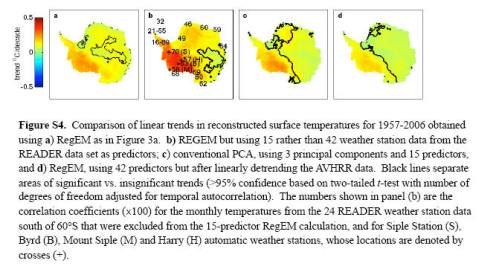
Update2: The Steig Corrigendum failed to replace their incorrrect SI Figure 4. Here is the original SI Figure 4.

Here is a corrected version as calculated by RomanM below.

Dr Phil, Confidential Agent

Recently, Philip Jones of CRU (Climatic Research Unit) claimed to have entered into a variety of confidentiality agreements with national meteorological services that prevent him from publicly archiving the land temperature data relied upon by IPCC.

Unfortunately, Jones seems to have lost or destroyed the confidentiality agreements in question and, according to the Met Office, can’t even remember who the confidentiality agreements were with. This doesn’t seem to bother the Met Office or anyone in the climate “Community”. This sits less well with Climate Audit readers, many of whom have made FOI requests for agreements between CRU and other countries throughout the world.

Because Jones is having so much trouble remembering who he made confidentiality agreements, we here at Climate Audit, always eager to assist climate scientists, are happy to do what we can to help Jones’ memory. I’ve spent some time reviewing Jones’ publications on the construction of the CRU_Tar index – in particular, Jones et al (1985); Jones (1994); Jones and Moberg (2003) and Brohan et al (2006). These contain interesting and relevant information on the provenance of Jones’ information and provide helpful clues on potential confidential agreements.

Jones insists on the distinction between academics and “non-academics” being scrupulously observed. I honored Jones’ demand that this distinction be observed by using his full academic title, Dr Phil, in the title, but, in the rest of the post, for the most part, I will refer to him more informally merely as Jones.

CDIAC

Jones has spent much of his academic career as a sort of temperature accountant. Commencing in the early 1980s, he collected station data and compiled averages – a useful enterprise, but surely no more than accounting.

In 1982 following the Three Mile Island incident and rising anti-nuclear sentiment, the US Department of Energy under the Reagan administration established the Carbon Dioxide Information Analysis Center (CDIAC), described by Wikipedia, as “the organization within the United States Department of Energy that has the primary responsibility for providing the US government and research community with global warming data and analysis as it pertains to energy issues.”

Wikipedia observes that CDIAC’s “present offices are located within the Environmental Sciences Division of Oak Ridge National Laboratory”. In fact, CDIAC’s offices have been at Oak Ridges either since its foundation (or closely so.) Oak Ridges’ main business is nuclear.

One of CDIAC’s first enterprises was its support of a world temperature index. As agents for this enterprise, they contracted Raymond Bradley, Thomas Wigley and Jones, all of whom become prominent figures in the IPCC movement. CDIAC published a “climatic data bank” of station temperatures in 1985 (Bradley et al 1985), the construction of which was described in Jones et al 1985a, 1985b, which described the data as “DOE” data. The first version was made available in print and diskette form, but a version from the late 1980s remains online at the CDIAC website. Jones et al 1985 descibed a data set with 1873 stations (1584 – NH; 289 – SH; 16- Antarctic); the ndp020r1 online version (circa 1990) has 1881 stations.

Here is a short clip of a contemporary confidential agent going to his work place, perhaps CDIAC, perhaps a front organization.

If Jones, as confidential agent for CDIAC in the 1980s, entered into confidentiality agreements with shadowy meteorological organizations and shady temperature data brokers around the world, he immediately breached such agreements by turning the data over to CDIAC, who published the station data both in print in 1985 and online. None of the shadowy meteorological organizations seems to have objected to any breach of contract by Jones.

More likely, there were no confidentiality agreements in this period. Jones et al 1985 does not describe any provenance of data from mysterious NMSs (national meterological services). Instead, it describes far more mundane provenance: by digitizing various editions of the Smithsonian’s World Weather Records and similar data from NCAR.

Jones(1994)

The first major update of the Jones data set was described in Jones (1994). Jones(1994) reported the continued financing of the CRU temperature index by the U.S. Department of Energy. The connection to the U.S. nuclear laboratories was less overt, with financing now attributed to the Atmospheric and Climate Research Division (Grant DE-FG02-86ER60397), attenuating the connection to the nuclear laboratories, though the archiving of gridded data at CDIAC, Oak Ridges was noted.

Jones (1994) referred to the use of 2961 stations; the next update (Jones and Moberg 2003) provided the additional information that the Jones (1994) dataset contained over 3900 stations, “of which 2961 stations were used in the gridding”. (The difference presumably arising from the availability of enough measurements in the reference period to qualify the series.)

A version of the Jones (1994) data set, vintage 1996, was made available at the CRU website (entitled cruwlda2.zip) and was publicly available from that time until July 31, 2009, when CRU purged their public data directories. For most of this period, there was a link from the CRU Advance-10Kwebpage (E.U. project number ENV4-CT95-0127) to cruwlda2.zip, evidencing that the data was intentionally placed in a public directory. On a few occasions, downloading of cruwlda2.zip has been reported by third parties.

Thus, if Jones entered into confidentiality agreements in respect to the Jones (1994) data set, once again, these agreements were promptly ignored.

It is more likely that there were no relevant confidentiality agreements from this period. Jones (1994) stated that the new stations were said to arise partly from additional information from stations in the extended network providing enough data to create a 1961-90 reference period (and thereby qualify the station for inclusion in gridding) and partly from “a number of projects e.g. Karl et al 1993 (BAMS)”, the latter including the Russia, China and Australia collections collated into GHCN. Jones (1994) did not mention the direct receipt of data from national meteorological organizations or international temperature data brokers/traders, shadowy or otherwise.

Jones and Moberg 2003

The next major update is described in Jones and Moberg 2003. Like the earlier versions, it was funded by the the U.S. Dept. of Energy (Grant DE-FG02-98ER62601). This time, Oak Ridges wasn’t mentioned anywhere.

Jones and Moberg 2003 reported the use of 5159 station records, of which 4167 had enough 1961-90 data to provide a reference period. Whereas the 1985 and 1994 editions contained no reference to direct dealings with national meteorological organizations (indeed they describe nothing much more than digitization of existing paper records or collation of GHCN sources), Jones and Moberg 2003 reported direct dealing with 7 national meteorological organizations:

CRU has collected a number of temperature records through direct contacts with the NMSs in Algeria, Croatia, Iran, Israel, South Africa, Syria, and Taiwan. Many of these records cover only the period 1961–90, but others extend over the entire twentieth century. Data for the whole of Australia for 1991–2000 have also been collected through direct contacts.

and later (also see Table 1):

CRU has received data from a number of countries through direct contacts with the respective NMSs. Records for 54 stations that were not represented in Jones were now included. Data for an additional 19 stations already represented in Jones were merged with priority for the NMS source. Most of these NMS records came from Iran, Algeria, Taiwan, Croatia, Israel, South Africa, and Syria. The merging of the NMS data was made after those from NHJ had been merged. As some stations were represented both in the NMS and NHJ data, the priority during merging was sometimes given to the data from NHJ rather than to data originating from Jones.

It’s an interesting list of NMSs. In other cases (Syria, Taiwan), CRU has some stations not represented in GHCN. In other cases (Iran, Algeria, Croatia, South Africa), there is an almost total overlap with GHCN IDs; however, for a number of stations, the Jones version is more extensive than the GHCN version, especially for Iran where CRU has an especially complete record. In this instance, the totalitarian regimes of CRU and the Ayatollah were apparently in complete agreement on the need to avoid public scrutiny. As to the confidentiality agreement between CRU and the Ayatollah, I guess that it was Burn after Reading.

Jones and Moberg (2003) also reported the acquisition of data on presumably conventional terms from less colorful regimes. They reported the use of new NORDKLIM data developed by the non-totalitarian regimes of Denmark, Sweden, Finland, Norway, Iceland, the United
Kingdom, Ireland, the Netherlands, and Belgium, as well as new datasets from non-totalitarian regimes in Canada and Australia.

Regardless of any possible confidentiality agreements, once again, CRU archived a near-contemporary version of the Jones and Moberg station data in early 2003, shortly after publication of Jones and Moberg 2003. The datasets newcrustnsall.dat and newcruextus.dat provide a combined total of 5070 stations, within 2% of the reported count of 5139 – pretty close when the Team is counting.

This dataset remained online until July 27, 2009, when it was purged by CRU. Unlike cruwlda2.zip, there were no links from CRU webpages to these datasets. Indeed, as we’ve discussed on previous occasions, both Dr Phil and the FOI officers at CRU and the Met Office on the one hand and people seeking copies of the Jones and Moberg data on the other seem to have been unaware of the existence of this data set until the connection of newcrustnsall.dat and newcruextus.dat to the long sought CRU station was reported at Climate Audit last month.

Brohan et al 2006

Brohan et al 2006, the next edition, reported that the development of the land station data set had been supported for the past 27 years by the US Department of Energy:

This work was funded by the Public Met. Service Research and Development Contract; and by the Department for Environment, Food and Rural Affairs, under Contract PECD/7/12/37. The development of the basic land station dataset has been supported over the last 27 years by the Office of science (BER), U.S. Department of Energy; most recently by grant DE-FG02-98ER62601.

They reported that the Jones and Moberg data set has “been expanded and improved for use in the new dataset”. It described the use of 4349 stations – I presume that this count corresponds to the 4167 in Jones and Moberg 2003 which had enough 1961-90 data to provide a reference period, rather than the 5159 overall total. As a result of FOI actions, a list of stations was provided in 2007 here, which reduced the count by 211 from 4349 to 4138. The associated webpage explained the reduction as follows:

The 4138 total is lower than the 4349 value given as the starting point for Brohan et al. (2006) and used in the latest IPCC Report. A small number of stations have been removed during Brohan et al. (2006) because of the presence of duplicate data and insufficient coverage for the period 1961-90.

“Duplicate” data mostly covers the inclusion of the same station in two different sources. For example, Jones 1994 included many USHCN stations under WMO numbers. Jones and Moberg 2003 added in the USHCN network with only a cursory effort to check for duplication – something that is a bit laborious, but only a few days work. As a result, there was extensive duplication. Most of the 211 duplicates removed for the webpage are USHCN stations. However, despite this belated check for duplicates carried out for the FOI response, quite a few duplicates still exist.

Although Brohan et al 2006 reported an “expanded” network, the new total of 4138 is lower than the count of Jones and Moberg 2003 stations in use (4167), though I presume that the Jones and Moberg count is inflated by 211 duplicates removed in the subsequent count. Brohan reported new stations were added for Mali, the Democratic Republic of Congo, Switzerland and Austria. Reported counts of 29 Mali stations and 33 Congo stations cannot be reconciled on existing information with much lower counts in the available listing.

While Brohan et al 2006 did not specifically attribute the provenance of the new data to direct contact by CRU with national meteorological organizations, this seems possible.

Confidentiality Policy

If one is trying to narrow down the search for the lost CRU confidentiality agreements, it seems to me that the logical place to start is with the following nine countries: Iran, Algeria, Taiwan, Croatia, Israel, South Africa, Syria, Mali, Congo. Did Dr Phil enter into confidentiality agreements with all or some of these nine countries? If so, what are the terms? And why are these agreements “lost”?

And exactly when were these agreements entered into? Our analysis shows that these agreements are not hoary old agreements from early Oak Ridges-CDIAC days, but were made well within the IPCC period. As a long-time IPCC hand, Jones knew of the IPCC commitment to “openness and transparency”.

Did Jones seek approval from an advisory board or some other form of independent oversight prior to unilaterally entering into confidentiality agreements with various totalitarian (and other) regimes? If these few confidentiality agreements are sufficient to poison public disclosure of the entire database (as CRU and the Met Office now argue), how was Phil Jones able to poison the public availability of the database through a few seemingly unsupervised confidentiality agreements?

UPDATE: As a closing thought (h/t reader below), recent CRU efforts to sanitize their public directories were perhaps anticipated by another confidential agent’s Cone of Silence:

"Unprecedented" Data Purge At CRU

On July 31, 2009, the purge of public data at CRU reached levels “unprecedented” in its recorded history. Climate Audit reader Super-Grover said that the data purge was “worse” than we expected.

On Monday, July 27, 2009, as reported in a prior thread, CRU deleted three files pertaining to station data from their public directory ftp://ftp.cru.uea.ac.uk/.
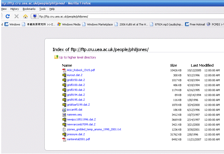
The next day, on July 28, Phil Jones deleted data from his public file – see screenshot with timestemp in post here, leaving online a variety of files from the 1990s as shown in the following screenshot taken on July 28, 2009.

The following day, the following listing of station data available since 1996 (discussed in my post CRU Then and Now) was deleted from public access: ftp://ftp.cru.uea.ac.uk/projects/advance10k/cruwlda2.zip, though other data in the file remained.

This morning, everything in Dr Phil’s directory had been removed.

This is part of a broader lockdown at CRU. Ian Harris, Dave Lister, Kate Willett, Tim Osborn, Dimitrios, Clive Wilkinson and Colin Harpham all altered their FTP directories this morning. Only one directory (Tim Osborn -see below) has added material.

Revisiting the Advance 10K webpage this morning, all Advance 10K data was deleted from their FTP site. None of the Advance 10K data links at http://www.cru.uea.ac.uk/advance10k/climdata.htm work any more.

If you go to the directory page ftp://ftp.cru.uea.ac.uk/projects which formerly hosted ftp://ftp.cru.uea.ac.uk/projects/advance10k directory, it now contains only two directories between Sept 1999 and the present, both dated 8/1/2008, but containing data from 2001.

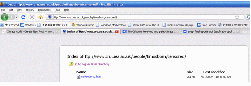
On July 31, 2009 at 10:41 am, Tim Osborn published a webpage entitled “controversy.htm”. It is located in a folder entitled ftp://www.cru.uea.ac.uk/people/timosborn/censored/ and the webpage ftp://www.cru.uea.ac.uk/people/timosborn/censored/controversy.htm itself is of course censored. [Update: Later on July 31, Tim Osborn, obviously a faithful Climate Audit reader, censored the censored folder and even the existence of the censored folder (and the controversy webpage) is now censored.]

I presume that the data has not been totally destroyed, only that, after many years of public availability, it has been put under lock and key. It’s as though CRU is having a collective temper tantrum.