Another Absurd Lewandowsky Correlation

Lewandowsky’s recent article, “Role of Conspiracist Ideation” continues Lewandowsky’s pontification on populations of 2, 1 and zero.

As observed here a couple of days ago, there were no respondents in the original survey who simultaneously believed that Diana faked her own death and was murdered. Nonetheless, in L13Role, Lewandowsky not only cited this faux example, but used it as a “hallmark” of conspiracist ideation:

For example, whereas coherence is a hallmark of most scientific theories, the simultaneous belief in mutually contradictory theories—e.g., that Princess Diana was murdered but faked her own death—is a notable aspect of conspiracist ideation [30].

However, this example is hardly an anomaly. The most cursory examination of L13 data shows other equally absurd examples.

One of the more amusing ones pertains to one of Lewandowsky’s signature assertions in Role, in which he claimed, echoing an almost identical assertion in Hoax, that “denial of the link between HIV and AIDS frequently involves conspiracist hypotheses, for example that AIDS was created by the U.S. Government [22–24].”

Lew reported a correlation of -0.111 between CYAIDS and CauseHIV, citing this correlation (together with negative correlations related to smoking and climate change) as follows:

The correlations confirm that rejection of scientific propositions is often accompanied by endorsement of scientific conspiracies pertinent to the proposition being rejected.

However, as with the fake Diana claims, Lewandowsky’s assertions are totally unsupported by his own data.

In the Role survey (1101 respondents), there were 53 who purported to disagree with the proposition that HIV caused AIDS (a vastly higher proportion than in the climate blog survey – a point that I will discuss separately). Of these 53 respondents, only two (3.8% of the 53 and 0.2% of the total) also purported to believe the proposition that the government caused AIDS. It is therefore simply untrue for Lewandowsky to assert, based on this data, that denial of the link between HIV and AIDS was either “frequently” or “often” accompanied by belief in the government AIDS conspiracy. It would be more accurate to say that it was “seldom” accompanied by such belief. Although Lewandowsky did not mention this, both of the two respondents who purported to believe this unlikely juxtaposition also believed that CO2 had caused serious negative damage over the past 50 years.

Lewanowsky’s assertion in Role about a supposed link between denial of a connection between HIV and AIDS and a government AIDS conspiracy had been previously made in Hoax not just once, but twice:

Likewise, rejection of the link between HIV and AIDS has been associated with the conspiratorial belief that HIV was created by the U.S. government to eradicate Black people (e.g., Bogart & Thorburn, 2005; Kalichman, Eaton, & Cherry, 2010)…

Thus, denial of HIV’s connection with AIDS has been linked to the belief that the U.S. gov¬ernment created HIV (Kalichman, 2009)

However, Lewandowsky’s false claim received even less support in the survey of stridently anti-skeptic Planet 3.0 blogs. Even with fraudulent responses, only 16 of 1145 (1.4%) purported to disagree with the proposition that HIV caused AIDS, and of these 16, only 2 (12.5%) also purported to endorse the CYAIDS conspiracy. These two respondents were the two respondents who implausibly purported to believe in every fanciful conspiracy. Even Tom Curtis of SKS argued that these responses were fraudulent. Without these two fraudulent responses, the real proportion in the blog survey is 0. Either way, the data contradicts Lewandowsky’s assertion that disagreement with the HIV-AIDS proposition is “often” or “frequently” accompanied by belief in the government AIDS conspiracy at the climate blogs surveyed by Lewandowsky.

Even though there were even fewer respondents supposedly subscribing to the unlikely propositions in the blog survey, the negative correlation between CYAIDS and CauseHIV propositions was even more extreme: a seemingly significant -0.31, though only the two fake respondents purported to hold the two unlikely propositions.

Update: I’ve added some plots below to illustrate how Lewandowsky’s calculations of correlation go awry.

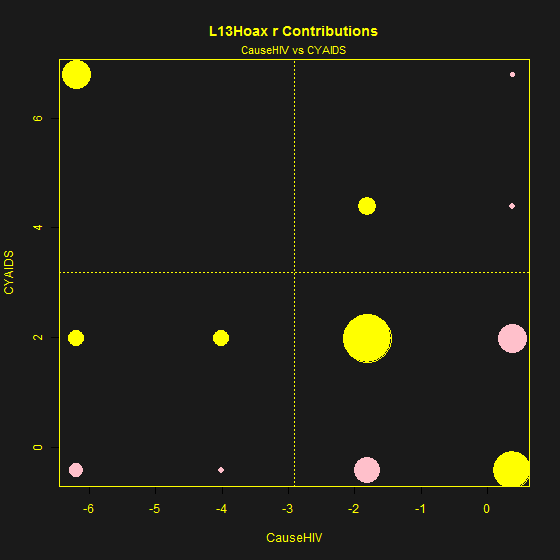
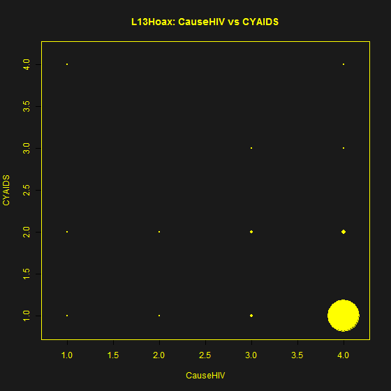
The contingency table of CauseHIV and CYAIDS for the L13Hoax data is shown below, with the size of each circle proportional to the count in the contingency table. Most of the responses are identical – thus the large circle. Because there are only two respondents purporting to hold the two most unlikely views, this is a very faint dot. A correlation coefficient implies a linear fit and normality of residuals: visually this is obviously not the case. There are a variety of tests that could be applied and the supposed Lewandowsky correlation will fail all of them.

CauseHIVvsCYAIDS_Hoax

If one goes back to the underlying definition of a correlation coefficent, it is a dot-product of two vectors. In the context of a contingency table, this means that the contribution of each square in the contingency table to the correlation can be separately identified. I’ve done this in the graphic shown below, since the points, while elementary, are not immediately intuitive in these small-population situations. For each square in the contingency table, I’ve calculated the dot-product contribution and multiplied it by the count in the square, thereby giving the contribution to the correlation coefficient (which is the sum of the dot-product contributions.) The area of each circle shows the contribution to the correlation coefficient: pink shows a negative contribution.

There are a few interesting points to observe. In a setup where nearly all the responses are identical and at one extreme, these responses make a positive contribution to the correlation coefficient. Responses in which the respondent strongly disagrees with CYAIDS but only agrees with CauseHIV or in which the respondent strongly agrees with CauseHIV but only disagrees with CYAIDS make a negative contribution to the correlation. Respondents with simple agreement with CauseHIV and simple disagreement with CYAIDS make a strong contribution to the correlation coefficient. The two (fake) respondents make a very large contribution to the correlation coefficent despite only being two responses.

CauseHIVvsCYAIDS r contributions_Hoax

A Scathing Indictment of Federally-Funded Nutrition Research

Edward Archer of the University of South Carolina, lead author of a scathing examination of U.S. federally-funded nutrition research, has written an even more scathing editorial in The Scientist (here) (H/t Margaret Wente of the Toronto Globe and Mail here.)

Some quotes:

We may be witnessing the confluence of two inherent components of the human condition: incompetence and self-interest

And while the self-correcting nature of science necessitates failure, the vast majority of nutrition’s failures were engendered by a complete lack of familiarity with the scientific method.

Rather than training graduate students in the scientific method, and allowing their research to serve the needs of society, the field’s leaders choose to train their mentees to serve only their own professional needs—namely, to obtain grant funding and publish their research.

But by not training mentees in the basics of science and skepticism, the nutrition field has fostered the use of measures that are so profoundly dissonant with scientific principles that they will never yield a definitive conclusion. As such, we now have multiple generations of nutrition researchers who dominate federal nutrition research and the peer review of that work, but lack the critical thinking skills necessary to critique or conduct sound scientific research.

The subjective data yielded by poorly formulated nutrition studies are also the perfect vehicle to perpetuate a never-ending cycle of ambiguous findings leading to ever-more federal funding.

Archer culminates with the following allegation (going much further than any of my comparatively mild critiques of climate scientists):

Perhaps more importantly, to waste finite health research resources on pseudo-quantitative methods and then attempt to base public health policy on these anecdotal “data” is not only inane, it is willfully fraudulent… The fact that nutrition researchers have known for decades that these techniques are invalid implies that the field has been perpetrating fraud against the US taxpayers for more than 40 years—far greater than any fraud perpetrated in the private sector (e.g., the Enron and Madoff scandals).

The study was not funded by the U.S. federal government, but by an “unrestricted research grant” from Coca-Cola.

This study was funded via an unrestricted research grant from The Coca-Cola Company. The sponsor of the study had no role in the study design, data collection, data analysis, data interpretation, or writing of the report.

I wonder if federally-funded nutrition scientists will respond with attacks on the Coke Brothers.

The Zen of Population (N=0)

Mann rose to prominence by supposedly being able to detect “faint” signals using “advanced” statistical methods. Lewandowsky has taken this to a new level: using lew-statistics, lew-scientists can deduce properties of population with no members. Josh summarizes the zen of lew-statistics as follows:

josh_Zero_Sum_scr

More False Claims from Lewandowsky

Another bogus claim from Lewandowsky would hardly seem to warrant a blog post, let alone a bogus claim about people holding contradictory beliefs. The ability of many climate scientists to hold contradictory beliefs at the same time has long been a topic of interest at climate blogs (Briffa’s self contradiction being a particular source of wonder at this blog). Thus no reader of this blog would preclude the possibility that undergraduate psychology students might also express contradictory beliefs in a survey.

Nonetheless, I’ve been mildly interested in Lewandowsky’s claims about people subscribing to contradictory beliefs at the same time, as for example, the following:

While consistency is a hallmark of science, conspiracy theorists often subscribe to contradictory beliefs at the same time – for example, that MI6 killed Princess Diana, and that she also faked her own death.

Lewandowsky’s assertions about Diana are based by an article by Wood et al. entitled “Dead and Alive: Beliefs in Contradictory Conspiracy Theories”. A few months ago, I requested the supporting data from Wood. Wood initially promised to provide the data, then said that he had to check with coauthors. I sent several reminders without success and eventually without eliciting any response. I accordingly sent an FOI request to his university, accompanied by a complaint under any applicable university data policies. The university responded cordially and Wood immediately provided the data.

The most cursory examination of the data contradicted Lewandowsky’s claim. One can only presume that Lewandowsky did not carry out any due diligence of his own before making the above assertion.

Continue reading

A New Climate Costumed Vigilante

A trivia question today for CA readers.
Continue reading

Rosenthal et al 2013

There has been considerable recent attention to Rosenthal et al 2013 (pdfpdf SI) :WUWT here, Judy Curry here, Andy Revkin here.

The article itself presents a Holocene temperature reconstruction that is very much at odds both with Marcott et al 2013 and Mann et al 2008. And, only a few weeks after IPCC expressed great confidence in the non-worldwideness of the Medieval Warm Period, Rosenthal et al 2013 argued that the Little Ice Age, Medieval Warm Period and Holocene Optimum were all global events.

Although (or perhaps because) the article apparently contradicts heroes of the revolution, Rosenthal et al 2013 included a single sentence of genuflection to CAGW:

The modern rate of Pacific OHC change is, however, the highest in the past 10,000 years (Fig. 4 and table S3).

In the Columbia and Rutgers press releases accompanying the article, this claim was ratcheted up into the much more grandiose assertion that modern warming is “15 times faster” than in previous warming cycles over the past 10,000 years (though the term “15 times faster” is not actually made in the peer reviewed article):

In a reconstruction of Pacific Ocean temperatures in the last 10,000 years, researchers have found that its middle depths have warmed 15 times faster in the last 60 years than they did during apparent natural warming cycles in the previous 10,000.

Rather than quoting the article itself, Michael Mann, an academic activist at Penn State University, repeated the claim from the press release in an article at Huffington Post entitled “Pacific Ocean Warming at Fastest Rate in 10,000 Years”.

However, both the claim in the press release and the somewhat weaker claim in the article appear to be unsupported by the actual data. Continue reading

The IPCC Southern Hemisphere Reconstructions

A question for readers: which of the following proxies are used to reconstruct past Southern Hemisphere temperature in the IPCC’s graphic (Figure 5.7b) showing SH reconstructions:

1. Graybill’s California strip-bark bristlecone chronologies
2. upside down and contaminated Finnish lake sediments
3. European instrumental temperature data
4. Antarctic ice core d18O isotope data covering the medieval period

Continue reading

More Moss from Miller

Gifford Miller’s most recent study on radiocarbon dates of Baffin Island moss has attracted recent publicity, including covers at Judy Curry, WUWT and Jim Bouldin, due to its claim to have demonstrated that the present is the warmest in 44000 years.

Over the past decade, Miller has been taking radiocarbon dates on moss exposed from receding glaciers/ice caps on Baffin Island. Up to his most recent study, these dates have been used to develop a chronology of ice expansion and recession. Miller’s sampling protocol focuses on “ice caps” rather (moving) glaciers and on short-lived moss (rather than longer-lived macrofossils). Miller assumes (reasonably enough) that the moss was engulfed by ice cap expansion – the expansion indicating a decline in temperature – and that the moss has not been subsequently exposed (since it degrades relatively rapidly upon exposure).

Miller’s article reports on 145 radiocarbon dates from recently-exposed moss, the vast majority of which are dated to the past two millennia, as shown in the histogram below of radiocarbon ages for the 135 Holocene dates (plus 10 pre-Holocene dates.)

miller 2013 radiocarbon histogram
Figure 1. Histogram of Radiocarbon Ages from Recently Exposed Baffin Island mosses (Miller et al 2013 GRL). Note: y-axis label is wrong. This is a histogram and y-axis is counts.

At the majority of locations, receding ice is exposing moss that was engulfed by Little Ice Age glacier expansion. At a sizable minority of locations, receding ice is exposing moss that was engulfed by earlier glacier expansions (especially first millennium AD and first millennium BC). These Holocene glacier expansions are consistent with other millennial evidence e.g. treelines moving south, ice core melt and oxygen isotopes. In an unpublicized part of Miller et al 2013, Miller estimated a secular lowering of glacier of 129 m/ 1000 years, with a 19th century low about 200 m below 20th century levels.

From the lowering of glacier lines, Miller estimated a reduction of about 2.7 deg C in summer temperature over the past 6000 years or so. Miller observed that estimates from CMIP5 climate models were much lower – about 1.1 deg C – from which he deduced that things were worse than we thought.

Some of the exposed samples are increasingly earlier in the Holocene, with the earliest Holocene sample at 4285 radiocarbon BP (calibrated 4900 BP). It should be noted that these dates do not coincide with peak Holocene warmth, dated to ~6000-7000 BP on much other evidence.

In addition to the 135 sites where Late and Holocene mosses have been exposed, Miller sampled 4 sites (10 samples) where the mosses were dated deep into the LGM or at or near the radiocarbon detection limit (~44000 years). It was on the basis of these samples that the warmest in 44000 years claim arose.

Curiously, this claim is remarkably similar to claims made by Lonnie Thompson in 2005 at Quelccaya (see CA discussion here, here here). In this case, “remarkably similar” means remarkably similar as normally understood, rather than as used in climate science. Thompson also based his claim on radiocarbon dates from moss (Distichia) exposed by receding glaciers. As in Baffin Island, the vast majority of Quelccaya radiocarbon dates were from the 4200BP and later, but there was at least one at the radiocarbon detection limit. Like Miller, Thompson hypothesized that this moss was evidence that temperatures were the warmest since the Eemian.

Since Thompson’s 2005 news release, there have been a couple of academic articles on the Quelccaya moss with Holocene dates, e.g. here which reported:

In this case, we can infer that not only one species but a community of plants occurred at a high-elevation location ∼5000 yr ago under likely warmer conditions.

However, I haven’t seen anything further about Thompson’s “Eemian” moss. If anyone knows anything more, I’d be interested. The outcome of Thompson’s “Eemian” moss seems like it would be relevant to the appraisal of Miller’s Eemian moss.

Miller et al provided the following helpful photo of the location from which one of the “Eemian” samples was taken. Miller commented that the moss is observed only in the immediate receding vicinity: the rock quickly becomes barren.
miller 2013 photo1
Figure 2. Photo of site of samples M10-B231v and B232v, dated at or near detection limit.

There are a couple of nearby locations at which the exposed moss from receding ice caps at slightly greater altitudes merely has Holocene dates. “Eemian” sample B231v is at 1395m altitude. However, samples B223v and B226v are both slightly higher and located nearby (with a km or two) along the same ridge, but the exposed moss is merely Holocene (~4200 BP). A question: How does one reconcile the supposed in situ continuity of the little “ice cap” in the vicinity of sample M10-B231v (1395 m) since 44000 BP with recession in the vicinity of nearby higher M10-B226v (1438 m)?

miller 2013 location map 1
Figure 3. Google Earth map in area of M10-231v.

Postscript: I’ve covered Miller’s work (relatively favorably) in the past – see here and here. Miller is a reputable scientist whose work rises above the data snooping, data mining and regression against increasing trends of self-opinionated verbiage (to borrow Briffa’s phrase) that is too prevalent in the field.

Much of Miller’s work has been the articulation of Late Holocene glaciation, up to and including its relative maximum in the Little Ice Age, from which numerous Baffin Island locations are still emerging in his recent study. Miller was coauthor of the Hvitavatn (Iceland) sediment series, with Miller attributing the Little Ice Age maximum of this proxy to cold, rather than warmth, and conversely for the Medieval period. As I noted in my coverage of PAGES2K, Kaufman and the PAGES2K authors used Miller’s series upside down, thereby attributing its 19th century maximum to warmth rather than cold. The PAGES2K Arctic reconstruction does not stand or fall on this error. However, it is one of relatively few series that show any Stick-ness and the other Stick contributors also have serious problems (e.g. contaminated sediments.)

hvitarvatn
Figure 4. Gifford Miller’s Hvitavatn series as used by PAGES2K Arctic.

Update: Oct 27. Andrews et al 1972 has an air photo on which the locations of B221v and B223v are shown. First, here is a google earth image looking east towards Broughton Island with sites marked – oriented to correspond to the 1972 air photo. The red pin shows the location of the ancient moss.

miller 2013 google view

Next here is the air photo from Andrews et al 1972.
andrews 1972 baffin

After discussing recent deterioration in summer temperatures, Andrews et al 1972 observed:

The evidence strongly suggests that glaciation of Baffin Island will herald the next glaciation of North America although the timing of such development is unknown. The climatic glacial mode may develop rapidly, but there is a lag of the order of 10,000 years in the subsequent buildup of a continental ice sheet… The recent climatic fluctuations in the area are on too short a timescale to be viewed with alarm. The main control on glacierization in eastern Baffin Island is snowfall, not temperature.

Co-authors of Andrews et al 1972 included Gifford Miller and Raymond Bradley.

Nick Brown Smelled BS

http://narrative.ly/pieces-of-mind/nick-brown-smelled-bull/ h/t Mosher.

Fixing the Facts 2

AR5 Second Order Draft (SOD) Figures 1.4 and 1.5 showed the discrepancy between observations and projections from previous assessment reports. SOD Figure 1.5 (see below as annotated) directly showed the discrepancy for AR4 without additional clutter from earlier assessment reports. Even though AR4 was the most recent and most relevant assessment report, SOD Figure 1.5 was simply deleted from the report.

Nor can it be contended that IPCC erroneously located the projections in SOD Figure 1.5, as SKS claimed here in respect to SOD Figure 1.4. The uncertainty envelope shown in SOD Figure 1.5 was cited to AR4 Figure 10.26. As a cross-check, I digitized relevant uncertainty envelopes from AR Figure 10.26 (which I’ll show later in this post) and plotted them in the figure below (A1B – red + signs; A1T orange). They match almost exactly. Richard Betts acknowledged the match here.

figure 1.5 SOD annotated
Figure 1. AR5 SOD Figure 1.5 with annotations showing HadCRUT4 (yellow) and uncertainty ranges from AR4 Figure 10.26 in 5-year increments (red + signs).

AR5 Figure 1.4
Having deleted the informative (perhaps too informative) SOD Figure 1.5, IPCC’s only comparison between AR4 projections and actuals is in the revised Figure 1.4, a figure that seems more designed to obscure than illuminate.

In the annotated version shown below, I’ve plotted the AR4 Figure 10.26 A1B uncertainty range in yellow. Unfortunately, Figure 1.4 no longer shows an uncertainty envelope for AR4 projections. Here one has to watch the pea carefully. Uncertainty envelopes are shown for the three early assessments, but not for AR4, though it is the most recent. All that is shown for AR4 are 2035 uncertainty ranges for three AR4 scenarios (including A1B) in the right margin, plus a spaghetti of individual runs (a spaghetti that does not correspond to any actual AR4 graphic.) From the right margin A1B uncertainty range, the missing A1B uncertainty range can be more or less interpolated, as I have done here with the red envelope. I matched 2035 uncertainty to the right margin and interpolated back to 2000 based on the shape of the other envelopes. The re-stated envelope is about twice as wide as the actual AR4 Figure 10.26 uncertainty envelope that had been used in SOD Figure 1.5. Even with this much expanded envelope, HadCRUT4 observations are at the very edge of the expanded envelope – and well outside the actual AR4 Figure 10.26 envelope.

figure 1.4 annotated
Figure 2. AR5 Figure 1.4 with annotations. The yellow wedge shows the uncertainty range from AR4 Figure 10.26 (A1B). The red wedge interpolates the implied uncertainty range based on the right margin A1B uncertainty range.

AR4 Figure 10.26

Richard Betts recognized that there was no location error in connection with AR4 projections, but argued (see here) that the comparison in AR5 Figure 1.4 was “scientifically better” than the comparison in the SOD figure which, as Betts acknowledged, was “based on” an actual AR4 graphic (AR4 Figure 10.26).

However, if one is comparing AR4 projections to observations, IPCC is obliged to compare to actual AR4 graphics. Figure 10.26 was properly recognized in the SOD as the relevant comparison. It was also cited in contemporary (early 2008) discussion of AR4 projections by Pielke Jr (e.g here) and Lucia (here here)

AR4 Figure 10.26 was a panel diagram, the bottom row of which (see below) showed projections for GLB temperatures under six emissions scenarios, including A1B, with the editorial AR4 comment that the models “compare favourably” with observations.
figure 10.26 panel
Figure 3. Bottom row of AR4 Figure 10.26 showing uncertainty ranges for GLB temperature for six SRES scenarios. Original caption (edits show information for bottom row): Fossil CO2, CH4 and SO2 emissions for six illustrative SRES non-mitigation emission scenarios … and global mean temperature projections based on an SCM tuned to 19 AOGCMs. The dark shaded areas in the bottom temperature panel represent the mean ±1 standard deviation for the 19 model tunings. The lighter shaded areas depict the change in this uncertainty range, if carbon cycle feedbacks are assumed to be lower or higher than in the medium setting… Global mean temperature results from the SCM for anthropogenic and natural forcing compare favourably with 20th-century observations (black line) as shown in the lower left panel (Folland et al., 2001; Jones et al., 2001; Jones and Moberg, 2003).

The next graphic shows the effect of AR5’s “re-stated” uncertainty range on Figure 10.26. The right margin uncertainty ranges of Figure 1.4 have been inset at the correct location, with the ends of the uncertainty range corresponding to 2035 values of the red envelope showing the re-stated uncertainty range. Despite the doubling of uncertainty in the AR5 restatement, recent HadCRUT4 values are at the very edge of the expanded envelope.

figure 10.26 with AR5 legend
Figure 4. Detail of AR4 Figure 10.26 with annotation. HadCRUT4 is overplotted: yellow to 2005, orange thereafter. Original reference period is 1981-2000; the 1961-90 reference period used in AR5 is shown on the right axis.

Conclusion
In the final draft document sent to external reviewers, SOD Figure 1.5 directly compared projections from AR4 Figure 10.26 to observations, a comparison which showed that recent observations were running below the uncertainty envelope. The reference period for the AR4 uncertainty envelope was well-specified (1981-2000) and IPCC correctly transposed the envelope to the 1961-1990 reference period used in SOD Figure 1.5.

IPCC defenders have purported to justify changes to the location of uncertainty envelopes from the three early assessment reports on the basis that IPCC had erroneously located them in SOD Figure 1.4. Thousands of institutions around the world routinely compare projections to actuals without making mistakes about what their past projections were. Such comparisons are simple accounting, rather than cutting-edge science. It is disquieting that such errors persisted into the third iteration of the documents and the final version sent to external reviewers.

But, be that as it may, there was no reference period error concerning AR4 projections or in SOD Figure 1.5. So reference period error is not a reason for the deletion of this figure.

Richard Betts did not dispute the accuracy of the comparison in SOD Figure 1.5, but argued that the new Figure 1.4 was “scientifically better”. But how can the comparison be “scientifically better” when uncertainty envelopes are shown for the three early assessment reports, but not for AR4. Nor can a comparison between observations and AR4 projections be made “scientifically better” – let alone valid in accounting terms – by replacing actual AR4 documents and graphics with a spaghetti graph that did not appear in AR4.

Nor is the new graphic based on any article in peer reviewed literature.

Nor did any external reviewers of the SOD suggest removal of Figure 1.5, though some (e.g. Ross McKitrick) pointed out the inconsistency between the soothing text and the discrepancy shown in the figures.

Nor, in the absence of error, is there any justification for such wholesale changes and deletions after the third and final iteration had been sent to external reviewers.

In the past, IPCC authors famously deleted data to “hide the decline” in Briffa’s temperature reconstruction in order to avoid “giving fodder to skeptics”. Without this past history, IPCC might be entitled to a little more latitude. However, neither IPCC nor its supporting institutions renounced such conduct or undertook avoid similar incidents in the future. Thus, IPCC is vulnerable to concerns that its deletion of SOD Figure 1.5 was primarily motivated to avoid “giving fodder to skeptics”.

Perhaps there’s a valid reason, but it hasn’t been presented yet.