Climate Audit

Back from a very pleasant Christmas.

A little while ago, I threaded an interesting comment by UC on Tamino’s criticism of Schwartz. As a blog management aside, I like having this kind of thread by others as it was a good comment and it was based on a careful analysis of third party literature. I have no problems threading material like this for discussion as it’s something that’s relevant and analytic and any subsequent discussion was on a relevant thread. My problem with the “thermo” discussions is mostly that too much of it has been too often unfocused, unrelated to primary literature and on irrelevant threads or unthreaded. I wanted to limit the topic until there were thread quality analyses.

Lucia has written a further analysis on the topic, which she’s posted at her own blog here. I’ve transferred some discussion from Unthreaded to the comments below.

Lucia builds on UC’s earlier analysis by making a distinction between how two quite different kinds of error can affect estimation of response time based on temperature data. One type of error occurs from making time averages of temperature data; a second time of error occurs from measurement errors in the temperature data.

Lucia observed that the Tamino-RC analysis argued that the Schwartz analysis was confounded by the first type of error (time averaging). Tamino produced a graphic showing that the GISS and simulated data did not match – presenting this a gotcha against Schwartz. Lucia shows that the effect of this particular class of error does not match the situation: she observes that this would yield a positive intercept for the intercept of time vs log(autocorrelation), whereas the actual result is negative. She observes:

If I were to plot Ln(Rθ) or a physical system with a linear response, that has been measure imprecisely, lack of precision in the measurements results in a negative intercept for the linear regression.

She observes, on the other hand, that the GISS situation nicely matches UC’s plots, thereby suggesting that measurement errors in the temperature data, rather than time averaging bias, accounted for the observed patterns.

My own feeling (and it’s not more than a feeling at this point) was that you couldn’t lean very heavily on response times calculated from the autocorrelations, regardless of whether one liked or disliked the answer.

Prior references on the topic include: Schwartz article; Tamino’s guest post at RC; Luboš comment, UC’s comment here, my report on Schwartz at AGU. In addition, Scafetta and West also consider response times from quite a different point of view (and are criticized by Rasmus at RC.)

Pielke Jr satirizes senior U.K. science adviser David King’s plea to women

“who find supercar drivers “sexy”, adding that they should divert their affections to men who live more environmentally-friendly lives.

King said:

“I was asked at a lecture by a young woman about what she could do and I told her to stop admiring young men in Ferraris,” he said.

“What I was saying is that you have got to admire people who are conserving energy and not those wilfully using it.”
…

“As soon as you come to the individual, however, they will buy a Ferrari, not because it is cheap to run or has low carbon dioxide emissions, but because young women think it is sexy to see men driving Ferraris. That is the area where a culture change is needed.”

UPDATE: King’s exposition invites satire and there have been some lively comments during the day. If you missed them, you’ve missed them because I’ve decided that we’ve had a little fun today, but I’m not going to preserve the repartee.

Ray PH reported at RC an AGU session describing the very interesting recent discovery of organic material disgorged from a retreating glacier N of 70N on the east coast of Greenland, with radiocarbon dates around the MWP.

To put things in perspective, I should first mention the talk by Tom Lowell, on work in collaboration with about a dozen other authors, concerning organic remains from the Istorvet Ice Cap in East Greenland. These are organic remains recently uncovered by the retreating glacier. Dating them tells you when the glacier had last retreated that far. Carbon-14 dates put the date of this earlier glacial retreat to between AD 800 and 1014, bracketing the time of the Norse colonization. Insofar as glaciers are primarily sensitive to temperature, that does indicate that in the Middle Ages this particular place, at least, was probably as warm as at present. It is an indication of some kind of regional warming in the area in the Middle Ages. Thus, if Greenland were taken in isolation, one couldn’t confidently say that what is going on there just now is completely unprecedented in the Holocene — at least not yet. However, as Tom would happily tell you, the Middle Ages were not as generally warm as the present, and Greenland shouldn’t be taken in isolation. It is the rapid melt in Greenland today, taken as one of a vast constellation of signatures of unusual warming, that gives one cause for concern.

The abstract for the AGU presentation entitled “Organic Remains from the Istorvet Ice Cap, Liverpool Land, East Greenland: A Record of Late Holocene Climate Change” by Lowell, T V, Kelly, M A, Hall, B., Smith, C A, Garhart, K,: Travis, S, and Denton, G H states:

Radiocarbon dates of emergent organic remains along the western margin of Istorvet ice cap (70.8°N, 22.2°W) indicate a time when the ice cap was smaller than at present. This ice cap, similar to others in east Greenland, exhibits “historic” moraines ~1-2 km in front of the presently retreating ice margins. At Istorvet, ice margin retreat has exposed a thin (~8 cm) organic horizon and in situ plant remains in bedrock cracks lie less than 10 m away from the present ice margin (453 m asl in 2006). Clusters of multi-species vegetation also were found on two nuntaks (to 719 m asl) located ~3 km from the historic drift limit. All organic remains were located in protected bedrock lees. On the west side of the ice-cap, vegetation is sparse but present at elevations near the ice margin. Both the ice cap geometry and the presence of overrun organic remains indicate past temperatures at least as warm as those at present. At Istorvet plant remains yielded 12 number of radiocarbon dates. These ages, when converted to calendar years, range from A.D. 400 to 1014, with the largest concentration from A.D. 800 to 1014. This work hones the conclusion of Funder (1978) who reported general climate deterioration since 800 BC. Moreover, it indicates warm conditons at this latitude at the time of Norse colonization of Greenland.

I emailed Dr Lowell asking both for a copy of the presentation and the proxy basis supporting Pierrehumbert’s statement that “Tom would happily tell you [that] the Middle Ages were not as generally warm as the present”. He promptly and cordially send me the first but not the second.

The dated organics are located in 4 sites near Scoresby Sund (70 45N 22W) on the east coast of Greenland. The reported dates are from a site near Istorvet, Liverpool Land. The majority are from 1040-1190 BP; a couple earlier 1380, 1590 BP. The dates are somewhat early relative to usual MWP concepts and Lowell is mulling over explanations and possibilities. The presentation states clearly that the organics are “within 280 vertical meters of ice cap summit” and located “where comparable modern assemblages do not exist”

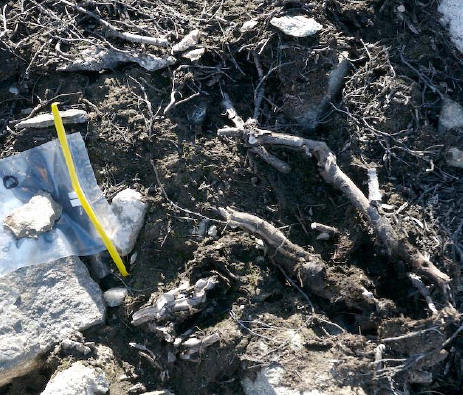
Here are a couple of pictures of the organics from the AGU presentation:

Two pictures of Istorvet Organic Material from Lowell et al 2007.

There are a few things to think about.

First, the dating seems a little earlier than one expects (or that Lowell expected.) In ocean sediment studies, one sees radiocarbon dates routinely adjusted for reservoir effects: could something similar arise here so that the dates are adjusted by, say, 200 years. Just a thought.

Second, over the past few years, when organic material is disgorged from retreating glaciers, people sometimes ask: where is the MWP material if it was supposedly as warm as the present? If one is looking for an example from Greenland with impeccable provenance, Lowell and coauthors have provided one. Whatever climate yielded the Istorvet organics would have applied to other parts of Greenland and the presence/absence of dated organics in any individual site would then be a matter of happenstance.

As to what amount of Arctic sea ice would be consistent with the observed MWP glacier retreat at Istorvet, east Greenland, I’m sure that we’ll hear about it.

In his comment quoted above, Pierrehumbert said that Lowell would “happily” say that the MWP was merely local to Greenland. As noted above, Lowell did not respond to my inquiry about this and so we are left to wonder about whether he actually holds this view and, if so, what the basis of this view is.

In 2000, Lowell wrote an interesting article for PNAS entitled: As climate changes, so do glaciers.

In respect to the MWP, Lowell stated:

A recent Northern Hemisphere temperature reconstruction indicates an oscillating temperature drop from A.D. 1000–1850 of about 0.2°C with a subsequent and still continuing warming of nearly 0.8°C (3).

You can easily guess what reference (3) was. So once again, we see the continuing application of MBH99 in hidden contexts: how do we know that “the Middle Ages were not as generally warm as the present”? MBH. It supposedly doesn’t “matter” but here it recurs once more to excuse inconvenient facts.

In Lowell 2000, the dominant view is that glacier changes occurred more or less concurrently around the world – a view illustrated by the Little Ice Age, the Younger Dryas and an episode prior to the Younger Dryas. Lowell stated:

Additional examples would confirm that, during the Little Ice Age, glacial systems expanded in concert and then withdrew together Because many glacial margins began retreat (A.D. ‘1850–1900) before the introduction of significant amounts of human-induced greenhouse gases, at least the initial part of the warming is a natural swing in the climate system. The continued warming and subsequent glacial retreat have uncovered buried forests in the Canadian Rockies (8) and elsewhere that are several thousand years old, which would require that these glaciers were once smaller than their present size. Such observations help define the range of natural climate variability.

and in connection with the earlier changes:

Do glacial systems respond to global climate changes? In addition to the global behavior during the Little Ice Age, two major glacial events at the end of the last Ice Age showing similar patterns from the mid-atitudes in both polar hemispheres and from the South Pacific and North Atlantic basins suggest that they do. … Before the Younger Dryas at the time of maximum continental ice volume (and hence the approximate low stand of global sea level; ref. 15), glacier systems made one final push…. along the eastern side of the Pacific, glaciers pulsed together, indicating a common climate forcing.

The entire tenor of Lowell’s article – that there were more or less synchronous changes – is inconsistent with the usual Team argument that the MWP was a dog’s breakfast of regional ups and downs, with negligible overall impact. To the limited extent that Lowell 2000 expressed an opinion on relative medieval-modern warmth, he merely cited MBH – hardly a high or independent authority. It’s possible that he holds this view and that he has alternative reasons for holding this view, but, to my knowledge there’s no evidence of him holding such views or providing an argued basis for them. So I don’t know whether Pierrehumbert had any basis for putting these words in Lowell’s mouth or whether he just assumed that Lowell would adhere to the RC party line.