Travel

I’m going to be a bit spotty online in the next 10 days as I’m visiting family and friends in Phoenix and Colorado Springs. Don’t ask me why a Canadian would leave a lake in Ontario for Phoenix in July. I have no answer other than perhaps Rumpole’s. I’m probably going to see at least one CA reader in Colo Springs. I’ll probably have time for a coffee in either spot if anyone wants to email me offline.

UPDATE: Steve has asked me to post a few items in his absence, such as interesting USHCN sites, so CA will not be without fresh material for the next 10 days. – Anthony

The New Mann Paper

The cat has finally dragged in Mann et al, Robustness of proxy-based climate field reconstruction methods, url 😉 Supplementary info. This article was first cited by the rather bilious 😈 Referee #2 for Burger and Cubasch , as though Burger should have been aware of its findings. The coauthors are the “independent” authors: Wahl, Ammann and Rutherford.

Perhaps responding in part to prior criticism, Mann has provided an extensive supplementary information, including code for many steps. (Whether the code works and whether it’s complete are different questions, but on the surface at least, it’s a big improvement.)

Jean S writes:

#99: It’s been already a while 😉 Supplementary info is available here.

Please, could someone check if I got this right:
Mann is reporting that his (in)famous North-American PC1 is orthogonal (r=0.011422767) to local temperature?
(MBHandMXDcorr.xls, MBH1980-sheet, row 89 and MBHHandMXDcorrNoInstr.xls, MBH1980-sheet, row 67)
Robustness paper:

UC writes:

Under the assumption of moderate or low signal-to noise ratios (e.g., lower than about SNR \approx 0.5 or “80 % noise”), which holds for the MBH98 proxy network as noted earlier, the value of \rho for the “noise” closely approximates that for the “proxy” (which represents a combination of signal and noise components).

Ah, that’s the way to estimate the redness of proxy noise. But isn’t this obvious, we have a model

P=\alpha T + n

and as \alpha is zero, we can estimate \rho of n directly from the proxy data 🙂

I haven’t had time to read it yet, but will try to do so soon, but a few quick comments.

I noticed that Mann has continued to use his PC methodology without changing a comma, notwithstanding the strong statement of Wegman that his PC methodology was simply “wrong” and the statement by the NAS panel that it should be avoided (And North’s testimony at the House E&C hearing that he agreed with Wegman) In effect, Mann is saying that, using his PC1, he can “get” a hockeystick not only with the Partial Least Squares regression of MBH98, but with the variation of RegEM (and I recall US pointing out some odd de-centering of his RegEM method.)

It’s one thing for Mann to keep using his PC methodology in the face of criticism from the Wegman and North panels, but why did the JGR reviewers acquiesce in the continued use of Mannian PCs? Pretty pathetic. Actually, it’s not just the JGR reviewers – Mann’s PC1 has been used recently by Osborn and Briffa 2006, Hegerl et al 2006 and Juckes et al – it’s as though the Team is brazenly showing solidarity with Mann to spite Wegman and others.

The word “bristlecone” is not mentioned anywhere in Mann’s new paper. So it’s a strange sort of “robustness” that Mann is proving. It’s already been agreed that, if you take the bristlecones out of the network, you can’t get a HS. So the original claim that the reconstruction is “robust” to the presence/absence of dendroclimatic indicators is false, although you won’t see a hint of that in this paper. Again, what were the reviewers doing? This has been a topical issue – why didn’t they ask Mann to consider it?

I checked Jean S’ comment about the PC1 correlation or lack of correlation and Jean S is right. The correlation of the MBH98 PC1 to the gridcell chosen here is 0.01 – not an imposing correlation for the one series that is essential to the reconstruction.

Here’s something else that’s amusing and shows Mann’s ridiculously perverse stubbornness and the ineptness of climate science referees. It’s been known for over 4 years that Mann mis-located a Paris precipitation in a New England gridcell (and Toulouse precipitation in South Carolina) and that the “Bombay” precipitation series does not come from Bombay. The mislocation of the Paris precipitation series was not corrected in the 2004 Corrigendum and, in the new SI, Paris precipitation is still shown with a New England location (“The rain in Maine falls mainly in the Seine.”) Mann and the mini-Manns duly report that the mis-located precipitation series has a positive correlation to New England gridcell temperatures. You’d think that they try to fix this sort of stuff at some point, but nope, the rain in Maine still falls in the Seine.

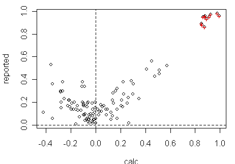
Update: I downloaded the reported correlation from the Mannian SI and then re-calculated correlations between the proxies in the AD1820 network and HadCRU3. Their SI stated:

Correlations were calculated between all 112 proxy indicators and both (1) local temperatures (average over the 4 nearest 5 degree lon x lat temperature gridpoints) … during overlapping intervals.

I then did a scatterplot comparing the reported correlations to the ones calculated using HadCRU3 – I used the single gridcell in which the record was located. The high correlations in the top right corner are correlations of actual temperature data to gridcell temperature – something that doesn’t seen like much of an accomplishment. Mann reported that all the correlations were positive, but I got no fewer than 60 out of 112 with negative correlations. Some prominent series e.g. GaspĂ© ring widths had negative correlations with HAdCRU3 gridcell temperatures.
mann01.gif

I presume, if a correlation was negative, that Mann just changed it to positive. For a few series, e.g. Quelccaya accumulation, there’s a plausible reason for this, but, in such cases, it would be better policy to invert the series ahead of time on a priori grounds. But there are some real puzzlers. For example, the GaspĂ© series (#53 – treeline11;St Anne) has a negative correlation (-0.11) with HadCRU3 gridcell, but Mann reports a positive correlation of 0.34. It’s hard to tell what’s going on – maybe Mann “inverted” negative correlations for reporting purposes, but they don’t invert the series for use in reconstructions.

4 More USHCN Stations

Anthony Watts writes in about 4 more USHCN stations: Continue reading

IPCC AR4: No skill in scientific forecasting

John A writes: After a brief search, I found the paper “Global Warming: Forecasts by Scientists versus Scientific Forecasts

This paper came to my attention via an article in the Sydney Morning Herald. It concerns a paper written by two experts on scientific forecasting where they perform an audit on Chapter 8 of WG1 in the latest IPCC report.

The authors, Armstrong and Green, begin with a bombshell:

In 2007, a panel of experts established by the World Meteorological Organization and the United Nations Environment Programme issued its updated, Fourth Assessment Report, forecasts. The Intergovernmental Panel on Climate Change’s Working Group One Report predicts dramatic and harmful increases in average world temperatures over the next 92 years. We asked, are these forecasts a good basis for developing public policy? Our answer is “no”.

Continue reading

The Al Gore Concert

I caught the start of the Al Gore concert last night in Sydney. It opened with a fat guy with white makeup beating his own drum. And it wasn’t even Al Gore.

The form of the concert reminded me of last weekend, Princess Diana concert except that it’s BIGGER, its consumption is more conspicuous and more lavish. Al Gore showed last year that he could use more electricity than 20 Americans and this year he showed that his concerts could use more electricity than 20 princesses. I guess that there must have been a form of competition between Al Gore and the Princess for stars. I wonder how many appear in both – I notice that Sarah Brightman is in both. Maybe some hung around London for a week watching Wimbledon.

Neither concert seemed very evocative of their causes. Elton John and Princess Diana – OK, I get that connection, but Kanye West and Princess Di? Somehow I doubt that many aspiring black rappers had little shrines to Princess Diana.

Today I pondered the linkage between Shakira and climate change. We used to hear about chaos and the butterfly effect – you know, the idea that when a butterfly flaps its wings in South America, it can change the chaos trajectory. Maybe this was what Al Gore was trying to illustrate – when Shakira sings about moving her hips and then shimmies for emphasis, this isn’ about music promotion, it’s a science lesson about the butterfly effect using a South American singer for authenticity.

But then over to Rihanna in Tokyo who was doing a ditty using umbrella as props. I think that the the message was that, with climate change, we would sometimes need umbrellas. But then she started shimmying as well, so maybe this was another lesson about the butterfly effect, but at a very profound level.

Regardless, both were big improvements over fat guys in white makeup beating their own drums. Anyway by this time, Wimbledon was on, so I could ponder more serious questions like whether Gasquet could challenge Federer or whether Djokovich had anything left in his tank after a 5 hour marathon match yesterday,

Review Comments on the "IPCC Test"

In a recent post, I’ve indicated that IPCC authors seems to have invented a “test” for long-term persistence that is nowhere attested in any statistical literature and, if I’ve interpreted what they’ve done correctly, appears to be a useless test.

Jean S and I have made a few references to the Review Comments on the “IPCC Test” and I thought that it would be interesting to collate them a little more systematically as they show the bullying tactics of IPCC authors and the total failure of review editors to ensure an adequate reply to reasonable comments.

Continue reading

Unthreaded #14

Continuation of Unthreaded #13

Multivariate Calibration

In calibration problem we have accurately known data values (X) and a responses to those values (Y). Responses are scaled and contaminated by noise (E), but easier to obtain. Given the calibration data (X,Y), we want to estimate new data values (X’) when we observe response Y’. Using Brown’s (Brown 1982) notation, we have a model

(1) Y' = -\alpha ^T + XB + E 

where sizes of matrices are Y (nXq), E (nXq), B(pXq), Y’ (1Xq), E’ (1Xq), X (nXp) and X’ (pX1). bf is a column vector of ones (nX1). This is a bit less general than Brown’s model (only one response vector for each X’). n is length of the calibration data, q length of the response vector, and p length of the unknown X’. For example, if Y contains proxy responses to global temperature X, p is one and q the number of proxy records.

In the following, it is assumed that columns of E are zero mean, normally distributed vectors. Furthermore, rows of E are uncorrelated. (This assumption would be contradicted by red proxy noise.) The (qXq) covariance matrix of noise is denoted by G. In addition, columns of X are centered and have average sum of squares one.

Continue reading

Central Park: Will the real Slim Shady please stand up?

Today, I’d like to discuss an interesting problem raised recently by Joe d’Aleo here – has the temperature of New York City increased in the past 50 years? Figure 1 below is excerpted from their note, about which they observed.

Note the adjustment was a significant one (a cooling exceeding 6 degrees from the mid 1950s to the mid 1990s.) Then inexplicably the adjustment diminished to less than 2 degrees …The result is what was a flat trend for the past 50 years became one with an accelerated warming in the past 20 years. It is not clear what changes in the metropolitan area occurred in the last 20 years to warrant a major adjustment to the adjustment. The park has remained the same and there has not been a population decline but a spurt in the city’s population in the 1990s.

I’ve spent some time trying to confirm their results and, as so often, in climate science, it led into an interesting little rat’s nest of adjustments, including another interesting Karl adjustment that hasn’t been canvassed here yet.

Update (afternoon): I’ve been able to emulate the Karl adjustment. If one reverse engineers this adjustment to calculate the New York City population used in the USHCN urban adjustment, the results are, in Per’s words, gobsmacking, even by climate science standards.)

Here is the implied New York City population required to justify Karl’s “urban warming bias” adjustments.

newyor5.gif
Continue reading

The New “IPCC Test” for Long-Term Persistence

In browsing AR4 chapter 3, I encountered something that seems very strange in Table 3.2 which reports trends and trend significance for a variety of prominent temperature series (HAdCRU, HadSST, CRUTem). The caption states:

The Durbin Watson D-statistic (not shown) for the residuals, after allowing for first-order serial correlation, never indicates significant positive serial correlation.

The Durbin-Watson test is a test for first-order serial correlation. So what exactly does it mean to say that the a test on the residuals, after allowing for first-order serial correlation, does not indicate first-order serial correlation? I have no idea. I asked a few statisticians and they had no idea either. I’ve corresponded with both Phil Jones and David Parker about this, trying to ascertain both what was involved in this test and to identify a statistical authority for this test. I have been unable to locate any statistical reference for this use of the Durbin-Watson test and no reference has turned up in my correspondence to date. (My own experiments – based on guesswork as to what they did – indicate that this sort of test would be ineffective against a random walk.)

The insertion of this comment about the Durbin-Watson test, if you track back through the First Draft, First Draft Comments, Second Draft and Second Draft Comments was primarily in response to a comment by Ross McKitrick about the calculation of trend significance, referring to Cohn and Lins 2005. The DW test “after allowing for serial correlation” was inserted by IPCC authors as a supposed rebuttal to this comment (without providing a citation for the methodology). I’m still in the process of trying to ascertain exactly what was done and whether it does what it was supposed to do, but the trail is somewhat interesting in itself.
Continue reading