RCS Homogeneity- Esper in Jaemtland

Starting with the first of my recent posts on Yamal, I raised the issue of whether the CRU 12 actually came from a homogeneous population to the subfossil population. This issue was related to the surprisingly small sample size of the supposedly “highly replicated” Yamal chronology, but is distinct. In his online response to Yamal posts, Briffa stated that they have “stressed” potential problems arising from “inhomogeneous” sources” in their “published work”.

Indeed, we have said so before and stressed in our published work that possible chronology biases can come about when the data used to build a regional chronology originate from inhomogeneous sources (i.e. sources that would indicate different growth levels under the same climate forcing).

Whether two populations are homogeneous is ultimately a statistical question. Consideration of this question as a statistical question has been blurred to date by the lack of understanding within the dendro community of the statistical issues involved in making a chronology (or within the statistical community of the difficult and interesting applied problems that dendros are trying to solve.) The disconnect is neatly illustrated by the references to Briffa and Melvin 2008, a highly technical article on standardization which nonetheless doesn’t include a single reference to an article or text by a non-dendro and which shows no awareness of how making a “chronology” ties into statistical literature on random effects (or how testing for population homogeneity relates to the statistical concept of “exchangeability”).

While Briffa’s articles occasionally contain caveats on population requirements for RCS standardization, I have been unable to locate any Briffa articles which he actually procedures for testing populations for homogeneity or the results of such tests, a lacuna that seems somewhat inconsistent with the idea that CRU has stressed this issue. In this instance, one wonders whether there is any practical difference between CRU stressing an issue and ignoring it.

While there doesn’t appear to be any relevant procedure in the Briffa corpus, Esper et al 2003 url does provide an on-point qualitative discussion of when two different populations can be combined in an RCS population (Tom P noted this in an earlier thread). It isn’t a formal test procedure, but it does provide a useful example (Jaemtland) where two populations were considered sufficiently distinct that they were not combined and does provide a basis for analysing Yamal homogeneity in a framework recognized by dendros.

In this post, I’ll provide a detailed description (and emulation) of the methodology described in Esper et al 2003, which, in another post, I will then attempt to apply to the “extended” Yamal data set recently presented by Briffa.

Esper’s example -see his Figure 8 – considered populations from two distinct sites: Jaemtland (swed023) and Trondelag (norw002), further distinguishing the Jaemtland site into two species PISY and PCAB. One attractive feature of this example as a precedent for analysing Yamal is that the Jaemtland population ends in the early 19th century, while the Trondelag population begins in the late18th/early 19th century, so that the techniques bear directly on the issue of population homogeneity between the Yamal subfossil and the “expanded” YAD-POR sites recently proposed by Briffa. To further accentuate the similarity, the Trondelag data set is a Schweingruber data set where each tree has two cores, while the Jaemtland data set is a non-Schweingruber data set with one core per tree.

Esper’s first step was to calculate age-dependence curves for each of the populations in question, plotting the resulting age dependence curves on the same quadrant. The following graphic shows the original Esper graphic, together with my emulation from available information (note Esper’s use of a biweight mean – which requires 4 samples). Esper observed that the (red) Trondelag (PISYsk) had a “significantly higher” growth rate and has a “rather different” slope than (black) Jaemtland. Esper’s comparison is qualitative, but nonetheless there is an obvious difference between the two age-dependence curves. One feels that this particular comparison could be worked up into a quantitative test (relatively easily if the comparison is between two negative exponential fits.)


Figure 1. Esper et al 2003 Figure 8B showing age dependence curves from two nearby sites. Left – original; right – emulation from Esper data obtained from Sciencemag. The core counts for Trondelag and Jaemtland match the reported core counts in E2003, but there is no available metadata showing which cores in swed023 are PISY and which are PCAB, the two species having been mixed in the archive. The Trondelag (PISYsk) curves should match exactly; while they are close, they don’t quite. Esper uses a biweight mean instead of a simple mean or median (this is OK.)

Esper demonstrated the impact of two non-homogeneous populations on an RCS chronology in his Figure 8D shown below at left versus my emulation shown at right, together with the core counts for Jaemtland (light gray) and Trondelag (dark gray). These show first of all that I’ve accurately emulated the key features of Esper’s methodology for this particular analysis. (Further comments below graphic.)

Figure 2. Left: Esper 2003 Figure 8D; right – Jaemtland chronology as used in Esper et al 2002, together with core counts. Light grey – Jaemtland; dark grey – Trondelag.

Look first at the early 19th century transition from Jaemtland to Trondelag data and the impact on the RCS chronology. Application of a one size fits all RCS method to this inhomogeneous population results in a inhomogeneity in the RCS chronology at the hinge point linking the two populations. Esper characterized the inhomogeneity as resulting in an “artificially shifted” mean in the early 1800s.

Esper stated that the inhomogeneity is caused by the

“rapidly growing [Trondelag] samples forcing the RCS spline [SM: would be the same for negative exponential] too high for the older, slower growing samples. This feature, namely the significantly deviating growth rates and growth decreases with aging of the Trondelag samples, indicates the existence of a different population in the sense introduced earlier. It also demonstrates the biasing effects of different populations and the fundamental requirement of the RCS method: sample homogeneity”.

There’s nothing in this paragraph that ought to be objectionable to any CA reader – it’s the sort of thing that we’re regularly concerned with. And it’s precisely the sort of thing that I’m wondering about at Yamal.

There are some other interesting features to this graphic. In the 13th century, the sample replication goes down to one core from Tornetrask, inserted into the data set as a bridge. The breakpoint in the RCS time series is pretty obvious. At the start of the record, replication falls below benchmark standards and again there is an obvious breakpoint.

In this particular analysis, Esper is at least attempting to analyse population homogeneity. In contrast, despite its length, the analysis in Briffa and Melvin 2008 fails to deal in any relevant way with the problem of population inhomogeneity (and other Briffa articles are even less helpful.)

When you have inhomogeneous populations, you can’t just add everything together. This is well understood in social science, where analysts have to take care to separate the effects of different factors. Esper’s Jaemtland-Trondelag example provides a foothold for trying to quantify population inhomogeneity within frameworks familiar to and accepted by dendros.

In a forthcoming post, I’ll apply these methods to both the Briffa 2000 Yamal data set and the “moved on” data set with some interesting and perhaps surprising results.

Script: multiproxy/esper/jaemtland.txt

Devi et al 2009

See comments introducing this extremely interesting article.

UPDATE: Since some readers are having routing issues downloading/reading this Devi et al paper, I have mirrored it here (PDF) for your convenience. – Anthony

Another Correction from Upside Down Mann

After a year of stonewalling, Mann has published an update at his “grey” Supplementary Information (not yet reported at PNAS) in which he acknowledges an “error” in his figure S8a as follows:

UPDATE 4 November 2009: Another error was found in the corrected Supplementary figure S8a from December 2008: The previously posted version of the figure had an error due to incorrect application of the procedure described in the paper for updating the network in each century increment. In the newly corrected figure, we have added the result for NH CPS without both tree-rings *and* the 7 potential “problem series.” Each of the various alternative versions where these sub-networks of proxy data have been excluded fall almost entirely within the uncertainties of the full reconstruction for at least the past 1100 years, while larger discrepancies are observed further back for the reconstruction without either tree-ring data or the 7 series in question, owing to the extreme sparseness of the resulting sub-network. The new figure can be downloaded here (PDF)

Continues discussion from here. See technical discussion of emulation of CPS at, for example, http://www.climateaudit.org/?p=4244 http://www.climateaudit.org/?p=4274 http://www.climateaudit.org/?p=4494 http://www.climateaudit.org/?p=4501. Continue reading

Taimyr and Yamal Location Maps

The following two Google maps show Taimyr and Yamal on consistent scales, together with Schweingruber sites in the area.

The Taimyr chronology in Briffa 2000, as you may recall, not only didn’t have HS, but had a notable divergence problem.

I’ve tried to accurately transcribe onto this location map the Naurzbaev 2002 sites (subfossil – white circles; living – three yellow icons), the Schweingruber sites (green). Briffa 2008 reported the addition of the Avam site (yellow labeled), about 400 km from the center of the Taimyr samples. They did not report the addition of the Schweingruber Balschaya Kamenka site relatively near Avam.

[This is what I’ve figure out so far. The precise network used in Briffa 2000 remains unreported. I can sort of guess by crosschecking the network in Esper 2002, obtained through quasi-litigation at Sciencemag, but there are some puzzles. Briffa 2008 contains no metadata as to which site any given core belongs to.]

There are some Schweingruber sites that seem far more obvious additions to Taimyr than Balschaya Kamenka: for example, the Schweingruber Kotuy River and Kotuykan River sites are slightly uphill from the Naurzbaev Kotuy River samples. The Schweingruber Novoja Rieka site seems to be almost co-located with a Naurzbaev location.

Why did Briffa go all the way to Balschaya Kamenka to add a Schweingruber site, while passing over the nearby sites? In the case of Yamal, where he also omitted a nearby site, Briffa said that they didn’t “simply” didn’t consider the nearby Khadyta River, Yamal site. Perhaps the same thing happened here.

Next here is a corresponding map for Yamal on precisely the same scale. Briffa’s online article made a bit of an issue of the fact that the Schweingruber Khadyta River, Yamal site was “slightly to the south” of the Porza and Yadaya sites – mentioning this not once but twice. However, Khadyta River is obviously far closer to the Porza and Yadaya sites than Avam or Balschaya are to Taimyr.

Polar Urals is also closer to Yamal than Avam is to Taimyr (I’ve got two slightly different latitudes for this site in my data collations – the present NCDC location has a latitude of 66 50N (but my collation of the Schweingruber locations once at NCDC but no longer there has a latitude of 67 50N). For present purposes, both locations are closer to Yamal than Avam is to Taimyr. Briffa said that he didn’t include Khadyta River in the Yamal RCS, because he “simply didn’t consider it”. He didn’t report on his deliberations regarding Polar Urals. Was it not included in the RCS because Briffa “simply didn’t consider it” or for some other reason?

These are elementary and obvious questions. Why are some sites included and some excluded? What are the scientific principles involved? Gavin Schmidt accused me of “randomly” picking a site off the internet, but that is not what I did. Given the precedent use of a Schweingruber site at Taimyr, I looked for the closest Schweingruber site to Yamal. In contrast, Briffa provided no guidance as to the basis for including one Schweingruber site rather than another. Did Briffa “randomly” pick Schweingruber sites to add – right now, we have no way of knowing?

Advocates at realclimate and elsewhere urge us to defer to Briffa’s choices. If Briffa’s articles are to be viewed as a branch of prophetic or oracular literature, then followers are, of course, entitled to defer to his choices.

However, if Briffa’s articles are to be considered as scientific articles, then the selection criteria need to be clearly stated and it should be possible to verify the choices. At present, I am not saying that there were no such rational criteria, only that the articles do not say what they were and, thus far, I have been unable to deduce what the criteria were.

Finnish TV

Jean S writes: Seems like Steve will be on Finnish TV next Monday 🙂
http://ohjelmat.yle.fi/mot/etusivu
I guess this image is from the CA headquarters 😉

Steve: Yes, this is indeed me at CA world headquarters.

9.11.2009 Klo 20:00
MOT: Ilmastokatastrofi peruutettu

Kööpenhaminan ilmastokokouksen lÀhestyessÀ kauhumaalailu ilmastokatastrofin seurauksista kiihtyy. Mediat tÀyttyvÀt uutisista, jotka kertovat jÀÀtiköiden sulamisista, meren pinnan noususta, myrskyistÀ ja tulvista, joita maapallon lÀmpenemisen vÀitetÀÀn aiheuttavan. LÀmpenemistÀ kuvataan ennen nÀkemÀttömÀksi.

MOT selvitti millaiseen tieteeseen vÀitteet ihmisen aiheuttamasta lÀmpenemisestÀ sekÀ sen dramaattisista seurauksista perustuvat. Osoittautui, ettÀ tutkimukset maapallon ennen kokemattomasta lÀmmön noususta viimeisten vuosikymmenten aikana eivÀt kestÀ lÀhempÀÀ tarkastelua.

MyöskÀÀn hiilidioksidipÀÀstöjen aiheuttaman lĂ€mpenemisen mÀÀrĂ€stĂ€ ei vallitse tieteellistĂ€ yksimielisyyttĂ€. Tuoreen MIT:n tutkimuksen mukaan hiilidioksidin kaksinkertaistuminen ilmakehĂ€ssĂ€ riittĂ€isi nostamaan maailman keskilĂ€mpöÀ korkeintaan 0,5, tietokonemallien ennustaman 2,5 – 6,0 asteen asemasta.

Toimittaja: Martti Backman

[Addition 11/9/2009 (Jean S): Transcript (in English) available here:

http://ohjelmat.yle.fi/mot/taman_viikon_mot/transcript_english ] archive

https://web.archive.org/web/20091113155332/http://ohjelmat.yle.fi/mot/taman_viikon_mot/transcript_english


Core Count in Phil Trans B

The Yamal reconstruction was introduced in Briffa 2000, a survey paper that did not include elementary information like core counts. As a result, users of the Briffa 2000 Yamal reconstruction (including Mann and Jones 2003, Moberg 2005, Hegerl 2007; D’Arrigo 2006, IPCC 2007, etc…) used it without any knowledge that the core counts did not meet RCS standards. In his recent online article, Briffa said that the closing portion of the Yamal results should be used “cautiously”. A Delayed Oscillator reader observed at Delayed Oscillatorthat this caveat should have been made clear in Briffa’s previous papers:

Briffa should have made clear in his papers that the post 1990 reconstruction was based on very few trees, and so should be “treated with caution”, as he explained in his recent web post.

Instead of agreeing with this obvious point, Delayed Oscillator argued that Briffa et al 2008 “shows sample size for each chronology”. Briffa et al 2008 would constitute notice only to users of this data after 2008 (such as Kaufman et al 2009), but does not constitute notice for users up to and including IPCC AR4. I wish that climate scientists would simply concede this sort of unwinnable point and focus on points that are interesting ones. If they don’t understand that notice in 2008 cannot be effective notice in 2000, it’s hard to have a sensible discussion.

But even the disclosure of Yamal sample size in Briffa et al 2008 is far from satisfactory. Here is their Table 1 reporting the number of samples during periods specified in the Table. In the -200 to 2000 period, Yamal is listed as having 611 samples, nearly double the number of samples for Avam-Taimyr (330), even though Avam-Taimyr had over 100 samples in 1990, while Yamal had only 10.

In the Phil Trans B measurement archive provided in Sept 2009, there are indeed 330 cores in the Avam-Taimyr sample, but for Yamal there are only 41% of the reported “611” samples. Phil Trans B Figure 3 shows core counts by year and looks like it uses the correct core count for Yamal (252 not 611.) The scale for core counts is inconsistent between panels, so that the relatively low closing counts for Yamal are not as clear as they might be.

If it weren’t for the incorrectly reported number of 611 samples for Yamal, Delayed Oscillator might be able to argue that Figure 3 constituted notice to post-2008 users and that Kaufman et al 2009 had satisfactory notice. However, under the circumstances, it is surely more than a little embarrassing that Briffa et al 2008 incorrectly reported the Yamal sample size as 611 rather than 252. I wonder where the figure of 611 came from??

Response to Briffa #2

As noted at CA last week, Briffa published a partial response to Yamal issues at the CRU website, one post discussing the impact of the Yamal chronology in various studies and another post discussing the Yamal chronology itself. For a response to Briffa’s online article on the impact of Yamal, I refer readers to last week’s analysis on this topic and my original post on this topic here. Briffa’s online articles on the Yamal chronology (and by “Briffa”, I include Melvin and Briffa’s associates) include a covering discussion here, a “sensitivity” analysis here and a data page here, which includes new measurement data and chronologies. (I’ll provide some tools and collations in due course.)

I am finalizing a lengthy post on population inhomogeneity which I’ll finish in a day or two. This extends previous discussion of population inhomogeneity in the “small” Yamal data set to the extended data set presented last week.

Today’s post is intended to clear away some side issues, showing in particular that Briffa did not endorse any of the arguments presented by realclimate or their followers. Not only did Briffa not endorse realclimate arguments, vituperative or otherwise, he specifically endorsed the legitimacy of CA-style sensitivity analyses. This may surprise both supporters and critics, but I submit that it is a fair reading of Briffa’s response as detailed below.

Indeed, it seems to me that Briffa did not actually contradict or rebut any specific empirical or statistical observation in any of my Yamal posts nor did he try to defend the aspects of Yamal methodology that were specifically criticised. Briffa’s defence was in effect the classic Team defence – “moving on”. Briffa argued that they can “get” a Stick from an expanded data set that was neither used in AR4 nor ever previously presented. Obviously, criticisms of the Yamal data set used in AR4 do not necessarily extend to the new data set; it has to be evaluated on its own merit. Equally however, the belated presentation of the “new” data set, whatever its merits may ultimately be, cannot “refute” or “rebut” criticisms of the existing data set. They may ultimately render discussion of the Yamal data set used in AR4 as moot, but they cannot “refute” any valid criticism.

Briffa’s online article, together with its accompanying data, although done quickly and presumably while Briffa is still recovering from a serious illness (I presume that Melvin was the main author), is a much more comprehensive presentation than anything in the “peer reviewed literature” about the Yamal chronology, which, despite the absence of even elementary information like core counts, was used by IPCC and multiproxy authors. While I think that there are important defects in the online article (especially the failure to demonstrate population homogeneity in the extended data set, a defect in the original chronology as well), nonetheless the online article is a big improvement over the previous literature and thus full credit to Briffa and associates for using online publication to improve the standard of presentation of the Yamal chronology from their previous defective presentations in academic journals.

With this lengthy preamble, I’d like now to examine the Briffa response in context of recent debate over CA posts that put the Yamal issue into play.

Khadyta River
Gavin Schmidt (and others) vituperatively criticized my use of Schweingruber’s Khadyta River data set to analyze Yamal RCS chronology sensitivity. Schmidt characterized me as merely using data “that [I] found lying around on the web.” However, Briffa stated that it was entirely appropriate to include Khadyta River in a Yamal chronology:

it is entirely appropriate to include the data from the KHAD site (used in McIntyre’s sensitivity test) when constructing a regional chronology for the area.

Briffa said that the only reason why they had not included this data themselves was that they simply didn’t think of it.

However, we simply did not consider these data at the time, focussing only on the data used in the companion study by Hantemirov and Shiyatov and supplied to us by them.

Gavin Schmidt was not the only critic to argue that using Khadyta River in a sensitivity test was some sort of violation of scientific principle. I haven’t noticed any withdrawal of such claims in the wake of Briffa’s response by Gavin Schmidt or others.

Sensitivity Testing of RCS Chronologies

Not only did Schmidt and others criticize the use of Schweingruber’s Khadyta River in sensitivity tests, they vituperatively criticized the very idea of a sensitivity analysis along the lines carried out here. However, Briffa’s response explicitly recognized and endorsed the sort of sensitivity study carried out at Climate Audit:

When using the RCS technique, it is important to examine the robustness of RCS chronologies, involving the type of sensitivity testing that McIntyre has undertaken and that we have shown in this example. Indeed, we have said so before and stressed in our published work that possible chronology biases can come about when the data used to build a regional chronology originate from inhomogeneous sources (i.e. sources that would indicate different growth levels under the same climate forcing).

Obviously, Briffa believes that he can work around the CA findings with the larger data set presented in his online article, but he recognized both the validity and importance of testing homogeneity and inhomogeneity. IMO, the new and larger data set is not out of the woods on inhomogeneity by any means; this is an issue that I will pursue in a technical post.

Abandoned Camp Sites
I had criticized the abysmally low 1990 core count in an RCS population, quoting Briffa’s own methodological observations in this context. I had also criticized the use of the corridor standardization subset (with its exclusive use of long cores) in an RCS program, again using Briffa’s own standards to criticize Yamal methodology. Some critics of CA counter-argued that 10 cores in 1990 was just fine and that the use of the corridor subset was just fine.

While Briffa did not explicitly concede either point, neither did he make any attempt to rebut my criticisms of the use of 10 cores in 1990 for RCS chronology or the use of a corridor subset of old trees for RCS chronology. He was completely silent on these issues.

Instead, his entire defence was one of “moving on”. Not that the prior methods were defensible, but that they could still “get” a similar result using a data set and methodology that were compliant with RCS standards.

In terms of camp site management, when campers move on, it would be nice if they tidied up the abandoned camp site i.e. denoting their agreement on issues that they were no longer defending – a practice which would avoid continued argument by third parties. However, the usual Team practice is to “move on” like nomads and leave abandoned camp sites in a total mess and unfortunately this happened once again here. This point about camp site etiquette reminds me of another frustrating aspect of Team debating style. Let’s suppose that the Team moves on to a new camp site and that they have proper hygiene and methodology at the new camp site. That doesn’t “refute” or “rebut” criticisms of their hygiene at the old camp site.

It will take more than a day or two to see if the hygiene and facilities at the new camp site are much of an improvement over the old camp site. We only learned of the new camp site last week. I think that Team supporters need to wait until the new camp site has been inspected before making a large down payment on the property.

False Accusations by Gavin Schmidt
Briffa took some care not to associate himself with untrue allegations made by Gavin Schmidt and others. Briffa observed that “subsequent reports” had misrepresented not merely his work, but also my original posts:

Subsequent reports of McIntyre’s blog (e.g. in The Telegraph, The Register and The Spectator) amount to hysterical, even defamatory misrepresentations, not only of our work but also of the content of the original McIntyre blog, by using words such as ‘scam’, ‘scandal’, ‘lie’, and ‘fraudulent’ with respect to our work.

While one understands that Briffa is more concerned about false allegations made against himself than false allegations made about me, it would have been constructive if Briffa had more explicitly disassociated himself from misrepresentations by Gavin Schmidt such as the following:

So along comes Steve McIntyre, self-styled slayer of hockey sticks, who declares without any evidence whatsoever that Briffa didn’t just reprocess the data from the Russians, but instead supposedly picked through it to give him the signal he wanted. These allegations have been made without any evidence whatsoever.

But at least Briffa did not perpetuate or endorse Schmidt’s false accusations and took pains to distinguish my remarks from remarks made by others. Even small steps are sometimes constructive.

Polar Urals and the Divergence Problem in West Siberia

On the minus side, Briffa totally avoided two critical reconciliations.

The online article made no mention whatever of Polar Urals and did not present any rationale for why the Polar Urals update has never been reported in “the peer reviewed literature” despite a shortage of millennial proxies. Nor did it present a rationale for using Yamal rather than Polar Urals (or a combination.) These questions remain even if they “move on” to a new Yamal data set.

In addition, the online article failed to reconcile the Yamal Stick (either old or new) with regional West Siberian results from the Schweingruber network (or Esper et al Glob Chg Biol 2009 discussed recently here [link]) showing a second-half 20th century decline in ring widths across a large population of sites. On numerous occasions, I’ve pointed to regional reconciliations as (IMO) critical in trying to advance paleoclimate beyond cherrypicking and data snooping and argued that a serious effort to investigate, analyze and reconcile this sort of regional reconciliation is what’s really required here.

Confirmation Bias
Briffa’s explanation of why the Khadyta River data wasn’t used is (IMO) an interesting example of confirmation bias.

Briffa agreed that there was nothing wrong with including the Khadyta River data in a regional chronology, but explained that this idea simply didn’t occur to them. Let me state clearly that I take them at their word and that I don’t have any reason to believe (nor do I think) that somewhere at CRU there is a “censored” directory with unreported adverse results with KHAD data together with verification r2 results.

On the other hand – and this is the precise point that instigated my Khadyta River analysis – over at Taimyr, where there was a particularly problematic divergence problem, the divergence problem led them to look for nearby data sets even though there was a lot more data at Taimyr than Yamal. At Taimyr, they ended up adding data from up to 400 km away, including from Schweingruber data sets contemporary with Khadyta River. Arguably, Yamal has a “divergence” in the opposite direction: its blade is unreasonably big. But this was the sort of result that they “expected” and they did not “think” about doing the same sort of procedure that they had carried out at Taimyr – look for nearby qualified sites. Had they done so, Khadyta River would have turned up right away for them, as it did for me (once I was aware that they had done this sort of thing at Taimyr.)

This seems like precisely the sort of confirmation bias that we’ve seen over and over again in this field. There seems to be more alertness to problems going the “wrong” way than there is to problems going the “right way”. The “residence time” of problems going the “right way” seems to be a lot longer than the “residence time” of problems going the wrong way, imparting a bias in reconstructions at any given time.

Data Availability
In a highly constructive departure from “peer reviewed” articles on Yamal, the article published on their webpage includes measurement data. Although the metadata is negligible (other than the location of the sample sites), the availability of measurement data accompanying the article in real time is a big improvement over prior defective presentations in the “peer reviewed literature” where there is no insistence on data archiving.

The big issue for this version (as it should have been for the last version) is population homogeneity – an issue that is not analysed or discussed in Briffa’s online article. I will post on that in the near future. For now, I’ll re-iterate the points at the start of this post: that the Briffa response accepts the legitimacy of the issues raised about Yamal at CA and that it does not endorse any of the attacks (or defences) advocated by Gavin Schmidt and realclimate supporters. Both constructive in different ways.

Sciencemag Enforces Data Archiving

As I surmised, Science has taken a dim view of Kaufman’s failure to provide data that was supposedly “publicly available” and most of the problems have now been dealt with. There are still a couple of issues though.

The three Finnish sediment series and one Canadian series have now been archived:
ftp://ftp.ncdc.noaa.gov/pub/data/paleo/paleolimnology/europe/finland/nautajarvi2005.txt
ftp://ftp.ncdc.noaa.gov/pub/data/paleo/paleolimnology/europe/finland/korttajarvi2003.txt
ftp://ftp.ncdc.noaa.gov/pub/data/paleo/paleolimnology/europe/finland/lehmilampi2007.txt
ftp://ftp.ncdc.noaa.gov/pub/data/paleo/paleolimnology/northamerica/canada/ellesmere/c2-1996.txt

In respect to the Canadian series, I’d like to specially note that Scott Lamoureux of Queen’s voluntarily sent me the data without being asked, when he learned that it had become an issue. I intended to comment favorably on this at the time; I regret that I didn’t do so right away, but do so now a few weeks later. He also said that he had sent the data to the paleo data bank a number of years ago, thought that it had been archived at one time and was surprised that it was not presently available (which he undertook to correct and has.)

The versions of four ice core series used in the Corrigendum are available in the pdf format increasingly used by paleos to prevent the use of turnkey scripts to access data. At least, they didn’t use the photo format of Esper et al 2009. The original data is here:
http://www.iceandclimate.nbi.ku.dk/data/Kaufman_etal_2009_data_29sep2009.pdf/

An ASCII collation is at CA here:
http://data.climateaudit.org/data/ice/kaufmansep09.dat

The D’Arrigo et al 2006 Gulf of Alaska chronology used by Kaufman remains unavailable. In addition, the Renland version as used in the original article remains unavailable – only the version used in the Corrigendum. The Corrigendum removes an adjustment reported in the peer reviewed article cited in Kaufman et al 2009 and it seems to me that Science should require the original version. Also that, if the Kaufman authors wish to alter the Renland series from the version presented in the original article, this should be presented to the referees and properly described in the Amended Supplementary Information.

At the time, I thought that it was pointless for Kaufman to think that Science would regard my data requests as anything other than well within their policies and that it was imprudent of him to force them to open the file. Sciencemag has done exactly what I anticipated. I’m sure that Kaufman is sulking a little about events, but he and other authors would be better off sulking less and archiving more. I sent a note thanking Science for their prompt attention to the above, reminding them that the D’Arrigo version is still unavailable and asking for the original Renland version.

I’ve also taken another crack at trying to get the D’Arrigo data, something that I originally attempted to obtain in 2005 as an IPCC reviewer. I sent a request to Colin O’Dowd, editor of JGR a couple of weeks ago, reminding him of my original 2005 request and reiterating my request for data, referring to very clear AGU policies on the matter. No answer or acknowledgement. Just as in 2005, when the only response to my similar request was IPCC threatening to remove me as a reviewer. This is a completely different attitude than Science, who are amazingly prompt in replying to my emails. I refreshed my request to O’Dowd, this time copying two members of the AGU Publications Committee, one of whom acknowledged the inquiry within minutes.

Esper et al 2009 on West Siberia

Esper et al (Global Change Biology, in press) “Trends and uncertainties in Siberian indicators of 20th century warming” is relevant to our present consideration of Briffa’s Yamal, which I will get to shortly. The cutline in their abstract declares in effect that the divergence problem is not as “bad as we thought”:

Despite these large uncertainties, instrumental and tree growth estimates for the entire 20th century warming interval match each other, to a degree previously not recognized, when care is taken to preserve long-term trends in the tree-ring data. We further show that careful examination of early temperature data and calibration of proxy timeseries over the full period of overlap with instrumental data are both necessary to properly estimate 20th century longterm changes and to avoid erroneous detection of post-1960 divergence.

However, it doesn’t seem to me that this is supported very convincingly by their data analysis. They analyze the (archived) Schweingruber to 1990-1991 plus a considerable number of recent measurements, all of which are unarchived – non-archiving seems to have become standard practice among Esper and Euro dendros. Esper et al also comment on the instrumental record, worrying about adjustments to a degree that would not be out of a place in a CA thread. Here are a few excerpts.

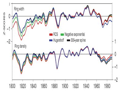
Here is an excerpt from Esper’s Figure 3, showing the effect of different standardization methods (Hugershoff, Negative Exponential, RCS and 300-year spline) on the average of over 70 chronologies. As you can readily see, on an overall basis, there is a decline in both RW and MXD for a very large population of Siberian sites since 1940 or so. Esper’s abstract and conclusions emphasize the fact that the post-1940 decline in the RCS version (red) is somewhat less than the post-1940 decline in the Hugershoff version (purple) – and also that the 19th century RCS rise is greater than the 19th century Hugershoff rise. However, in our consideration of Yamal, the slight difference in post-1940 decline is irrelevant: once again, the large population doesn’t show the huge Yamal rise. The issue, as stated on many occasions, isn’t just the “divergence” of Briffa’s Yamal chronology from Khadyta River, but its “divergence” from growth patterns throughout western Siberia – making one wonder about possible inhomogeneity in the Yamal population, an issue that I’ll return to.


Esper Fig. 3 Lower Panel Effect of tree-ring detrending… Lower panel shows the same arithmetic means (RCS) together with the mean timeseries derived from HUG, EXD, and SPL detrending. All timeseries were normalized over the 1881–1940 period. RCS, regional curve standardization; TRW, tree-ring width.

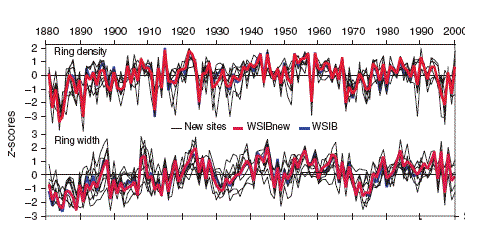
Esper specifically showed results from a “new” (and Euro-unarchived) west Siberian network, summarized in the next graphic. The “new” network ends up at a z-score in 2000 of almost exactly zero, while Briffa’s Yamal is exploring stratospheric multi-sigma deviations.


Esper Fig. 6. Updated WSIBnew tree-ring data and coherence with regional temperatures. Top panel shows the seven new MXD and eight new TRW RCS-detrended site chronologies together with their mean (WSIBnew) and the mean of all records in the WSIB clusters C1-3 (WSIB). While the latter extended only until 1990, WSIBnew reached 2000. Middle panel shows the WSIB and WSIBnew tree growth data scaled over the 1881–1990 (WSIB) and 1881–2000 (WSIBnew) periods to regional JJA temperatures. JJA and WSIB data have been decadally smoothed. Bottom panel shows the WSIBnew MXD and TRW timeseries together with JJA temperatures over the 1970–2000 period. Details on the updated WSIBnew sites, and all other tree-ring locations, are listed in supplementary Table S2. RCS, regional curve standardization; TRW, tree-ring width.

Esper also questions a variety of issues in the station histories, mentioning UHI, regional inhomogeneity in adjustment practices (see the Discussion and Conclusion for these) and GHCN adjustments. On regional adjustment to temperature records, they say:

In addition, the homogenization methodologies currently applied particularly in large-scale approaches, have difficulties in identifying and correcting for systematic biases that simultaneously affect data across larger regions (Parker, 1994; Frank et al., 2007a; Thompson et al., 2008). If we, for example, consider the substantial changes of instrumental summer temperatures that were recently applied to early station data in Europe and elsewhere (see both Frank et al., 2007a; Bohm et al., 2009, and references therein), it appears premature to solely use early temperature readings for proxy transfer and evaluation of DP in remote high latitude regions

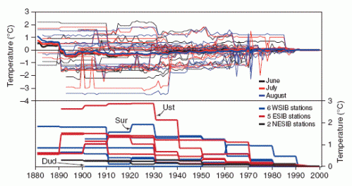
The top panel below shows a graphic displaying GHCN adjustments of the sort that I did here a couple of years ago in connection with Hansen’s Y2K problem, emphasizing that the adjustments are as large or larger than the temperature changes being measured (a familiar CA point.) In the caption to the bottom panel, he says: “Negative deviations were inverted, combined with positive values, and decadally averaged.” I don’t understand the purpose of this procedure and had enough needles in my eyes for a while.


Esper Fig. 8 Differences between raw and adjusted (GHCN) temperature station records. Upper panel shows the single June, July, and August adjustments of all 13 Siberian stations and their mean timeseries (bold). In the lower panel the adjustments were averaged to mean JJA mean timeseries and sorted by stations in WSIB, ESIB, and NESIB. Negative deviations were inverted, combined with positive values, and decadally averaged. Ust is Ust’-Maja, Sur is Surgut, and Dud is Dudinka (see Table S3).

For our present consideration of Yamal, the evidence from the Esper networks in western Siberia is one of declining ring widths in the last half of the 20th century. Briffa’s Yamal is an exception to this general pattern – a point that is not discussed or reconciled in Briffa’s response thus far. Esper cautions in respect to RCS standardization:

It seems important to note, however, that RCS-detrended data generally contain greatest uncertainties, require large datasets, and are prone to biases caused by inhomogeneous sample collections (Esper et al., 2002, 2003a). Particularly relevant to the Siberian data analyzed here could be biases due to (i) the tendency that the oldest trees often grow most slowly (Melvin, 2004; Esper et al., 2007b; Wunder et al., 2008), and (ii) the composition of data from only living trees and relatively homogeneous age-structure (Esper et al., 2007a, 2009). The former bias is likely more relevant for TRW than MXD – because of the greater amount of variance contained by the agetrend (Schweingruber et al., 1979) – and would ultimately increase positive long-term trends in RCS chronologies.

In his response, Briffa made no effort to defend the methodology of the original Yamal chronology beyond declaring that it was done in good faith, instead moving on to argue that they can “get” a similar chronology from a somewhat larger data set, as presented last week. The most important issue – as stated here and elsewhere by Esper – is the potential “bias caused by inhomogeneous sample collections”, an issue that I’ll consider in connection with the new Yamal data in a forthcoming post.

Rank Gavin Noise


William Connolley is still, shall we say, manfully pretending not to understand how sediments affected by bridge-building, ditches and agriculturally activity cannot be excellent temperature “proxies” if they correlate with NH temperature.

Amazingly, some of his readers, like PNAS editors and referees, take this sort of stuff seriously.

Just for fun, I’ve constructed an example that, IMO, contains the relevant features of the Tiljander example, combining a well known series with “rank Gavin noise”, defined here as two times log(1000) minus the log of the rank of Gavin among US names (somewhat modifying realclimate’s Gavin index, originally proposed by Lucia.)

As you see, it has a familiar hockey stick shape. It has an excellent correlation (.81; r2: 0.65) with HadCRU global temperature during the “calibration period” of 1954-2008 when Gavin ranks are available here .


Figure 1. “Proxy” plus Rank Gavin Noise

Readers are invited to identify the mystery proxy – which shouldn’t be too hard for CA readers.

While the example is constructed to be amusing, there is a fundamental point here – in general, Team methodologies assert without ever providing proof that “proxies” are a combination of “true temperature” plus white noise or low-order red noise.

The metaphor – and it is a metaphor – of “signal” and “noise” for sediment or tree ring series is one that troubles me and many other statistically oriented CA readers, however climate scientists to date have been totally unmoved by such concerns, seemingly having trouble understanding such elementary things as Mann’s misuse of the Tiljander series.

Obviously there’s a communications gap; maybe adding the concept of “rank Gavin noise” to noise repertoires of climate scientists will help bridge this gap.