Connolley Endorses Upside Down Mann

Kaufman’s grudging acknowledgement (see their draft Corrigendum) that they used the Tiljander proxies upside down has not convinced the Team that the identical orientation of the Tiljander proxies in Mann et al 2008 was also upside down.

There has been an active new round of debate in the blogs, with William Connolley endorsing Upside Down Mann. It seems that we are facing not simply an Upside Down Mann, but an Upside Down Team.

Roger Pielke Jr had opined hopefully that this concession would finally settle at least one small point in paleoclimate. Pielke said that “it looks like this dispute will in fact be resolved unequivocally through the peer-reviewed literature, which for all of its faults, is the media of record for scientific claims and counterclaims”. Pielke was obviously aware of the role of blogs (both Climate Audit and in Finland) in this dispute and was here focusing more on the fact that Kaufman was admitting the upside down use in a formal venue, rather than the role of the journals in extracting the admission from Kaufman. This point was misconstrued by Ben Hale here who interpreted Roger’s post as evidence that the Kaufman error had been detected and resolved by journal peer review and due diligence, when that’s not what happened at all. (I posted a comment at Hale’s to this effect.)

The debate over the relationship of blogs and Peer Reviewed Literature is one that Andy Revkin raised recently as well. And it’s one that’s playing out in a very interesting way in the recent Briffa commentary on Yamal, which, regardless of how this issue plays out, is, in my opinion, a more substantive and interesting bit of work of than any of his recent articles in the Peer Reviewed Literature, because it is accompanied on time by DATA, is technical and makes no effort at faux “originality”. (Obviously much more on this in the next week or two.)

Had matters been left with blogs debating the relative contributions of blogs and Peer Reviewed Literature in the settling of this small point, that would seem like the logical denouement of this sorry little episode.

But this under-estimated the propensity of the Team to engage in prolonged trench warfare on the most elementary and seemingly unwinnable points. A Pielke commenter argued that, under Mann’s methods, the “data can’t be upside-down”, adding that neither Pielke nor I were qualified to engage in such a debate anyway:

“Multivariate regression methods are insensitive to the sign of predictors”. Mann et al seem to be saying their methods are invariant to the data’s orientation – perhaps to linear translation? – anyway it means the data can’t be upside-down. Now if the mathematical interpretation placed on the data by their methods conflict with physical information from other sources, it does raise questions. Presumably the next sentences in Mann et al’s reply l refer to this, I can’t see anything in Kaufman et al that illuminates this and it would seem to require detailed knowledge of the field to judge the importance of these issues. And as you said, we (you, me, Steve McIntyre,…) are not professionally qualified to engage in the substance of such a debate.

Despite the worries of Pielke’s reader as to whether Pielke or I were sufficiently qualified to determine whether a series is going up or going down, I can assure the reader that I have enough experience in the stock market (both painful and otherwise) that I know the difference between whether things are going up or down, and I believe that even readers uninitiated into the mysteries of RegEM are capable of understanding the difference.

This comment at Pielke’s was praised by William Connolley, the Team’s representative at Wikipedia, in a recent post decrying Pielke. Connolley then vigorously supported Upside Down Mann in comments at both Pielke Jr and Ben Hale, where the matter has been discussed relatively briskly.

Mann’s use of the Tiljander sediments was originally discussed here on Oct 2, 2008, a post which discussed the multiple problems with Mann’s use of these proxies, summarized as follows:

In Mann et al 2008, there is a truly remarkable example of opportunistic after-the-fact sign selection, which, in addition, beautifully illustrates the concept of spurious regression, a concept that seems to baffle signal mining paleoclimatologists.

The issue with Mann’s use of the Tiljander proxies isn’t just that he used them upside down (which he did). The problem is worse than that. The Tiljander sediments are the combination of two unrelated processes: a presumably climatically driven process in which narrow sediments are interpreted by the authors as “warm” and thick sediments as “cold” and a nonclimatic process in which sediments are produced by ditches, bridges and farming.

Although the following point is not well understood by climate scientists (including, apparently, Connolley and Mann), a “reconstruction” at the end of the day is a linear combination of the proxies. While Peer Reviewed Literature does not require climate scientists to report these weights, in our dissections of reconstruction methodologies, this is the sort of thing that we keep track of.

Leaving CPS aside for a moment, Mann and his defenders say that, in a multiple regression setting, it doesn’t “matter” what the orientation of the series is going in to the meatgrinder. However, this ignores the relevant issue of what the orientation of the series is coming out of the meatgrinder. Connolley and Mann and others seem to assume that the meatgrinder can’t get it wrong. But this is not the case either in principle or in the particular case of the Tiljander sediments.

By examining the code to keep track of weights (as Jean S, UC and myself have done), it is possible to track the orientation of the Tiljander sediments into the final reconstruction and see whether the contribution of the Tiljander sediments to the reconstruction is inverse to the interpretation of the original authors or not. It is definitely and incontrovertibly upside down.

The reason why it is upside down is the spurious correlation between the nonclimatic sediments from bridges and farming and temperature, which confuses the Mannian meatgrinder algorithm. While I confirmed my understanding of the sediment interpretation by email with Tiljander, this is also clearly reported in the original article (See my original note on this).

As I’ve recounted at CA (most recently here), we reported these and other problems in our PNAS Comment. These comments are limited to 250 words, 5 references and no figures. This is far less detail than available in any blog post. Connolley’s most recent argument is that our PNAS Comment was insufficiently clear.

Perhaps Connolley is gradually realizing that the problem is not just the upside down proxy, but a package of issues including modern contamination and spurious regression. Needless to say, Connolley doesn’t blame Mann for making the errors, but blames me for not expressing these points clearly enough that even a climate scientist could understand them.

If he meant what you said, he could and should have said so.

Quite frankly, I’m baffled at what else I could have said. The issues seem very elementary to me and I don’t understand why they seem to difficult for climate scientists. Let me try one more analogy. As noted above, the Tiljander sediments are in a sense a “compound” of a climatic and nonclimatic process.

Consider a series defined as the difference between the incidence of the name Gavin (which increases strongly in the 20th century) and the Central England temperature (scaled to keep on the same page) and feed this into a Mannian meatgrinder. The Mannian algorithm will detect a strong correlation between the compound series and world temperature during the 20th century. In the “reconstruction” period when the Gavin effect wears off and is at a very low level, the compound series is the inverted temperature (upside down). The spurious regression results in the series being upside down in the reconstruction period.

As I said above, it’s not just that the series is used upside down; there’s a combination of problems, ones that, in my opinion, were fully described in posts on the topic (posts that are easily located merely by googling “Upside Down Mann” and following the links.)

For Connolley’s benefit, here is the Oct 2, 2008 post reprinted in its entirety (also see here for a most recent review). The issues are not very complicated. Continue reading

Briffa on Yamal Impact

Keith Briffa has a couple of posts today on Yamal – one discussing its impact in other multiproxy studies and the other on the Yamal chronology itself. His post on the Yamal chronology includes a careful consideration of various issues involved in the development of the Yamal chronology and is accompanied by an extensive archive of original data. The concurrent inclusion of data is to be commended.

It will take a little while to consider this as there’s a lot of data to assimilate. First, let me discuss the post on the impact, which I can do quite quickly.

Briffa considers three aspects of Yamal use: (1) in Osborn and Briffa 2006; (2) in IPCC 2007; and (3) in other multiproxy studies. He concludes:

Thus, with the exception of Briffa (2000), the reconstructions shown by the IPCC (Figure 6) either do not use the Yamal record or they combine the Yamal record with many others and this reduces their sensitivity to the inclusion of any individual records.

I disagree with this summary for several reasons outlined below.

I considered the impact of Yamal on other multiproxy studies in a CA post here, which is, unfortunately, not linked in the corresponding Briffa comment. There are many points of empirical agreement, but considerable differences in emphasis. The differences in emphasis are significant: I considered the use of both Yamal and strip-bark bristlecones/foxtails, identifying several “families” of reconstructions: a family in which strip bark bristlecones/foxtails were highly influential (but not Yamal); a family in which Yamal was highly influential (but not bristlecones); a belt-and-braces family in which both were used and which typically asserted “robustness” to removal of individual proxies; and a few odds-and-ends which were affected by other questionable proxies e.g. by the “cold” 11th century Polar Urals of Briffa et al 1995.

Yamal arose as an issue in the wake of our criticism of MBH, because of Team assertions that the Mann reconstruction was supported by various “independent” reconstructions. We observed (and this point has been also observed by Briffa in the past) that the “independent” reconstructions are not, in fact, “independent” because of their re-use of the same proxies over and over, especially strip bark bristlecones/foxtails (both directly and as Mann’s PC1). Strip bark has been the more contentious issue; as I noted in my prior post ( a point also made in Wegman 2006), many of these supposedly “independent” reconstructions use strip bark bristlecones. However, not all of them do. Yamal became important as an issue because it is influential in reconstructions that do not use bristlecones (Briffa 200, D’Arrigo 2006, Kaufman 2009). To the considerable extent that Briffa’s response to Yamal impact is that they can “get” a stick using strip bark, the response is, shall we say in Mannian-speak, a little “disingenous”.

Briffa’s statement contradicts empirical observations at CA 7229 in only a couple of places and, in each case, I can demonstrate that Briffa is wrong. Both errors are relevant.

First, Briffa said that Hegerl et al (2006) did not use Yamal, while I said that they did. Hegerl et al (Nature 2006) url does not list the series that it uses; the companion Hegerl et al 2007 url states:

the west Siberia long composite involved Yamal and the west Urals composite.

Precisely how Yamal is “involved” in the west Siberia long composite is not reported. I’ve been trying to get the exact versions used by Hegerl since fall 2005 and despite many emails (mostly involving Crowley) have thus far been unsuccessful. (As I’ve mentioned elsewhere, my original attempts to get this data led to IPCC WG1 Chair Susan Solomon threatening to expel me as an IPCC reviewer.) On the empirical point of whether Hegerl et al used Yamal, given the explicit statement in Hegerl et al 2007, it is my opinion that Briffa is wrong.

Second, as regards d’Arrigo et al, Briffa said that Yamal was used, though “possibly labelled as Polar Urals”. To use a Mannian term, it is “disingenuous” to say that it was “possibly” labelled as Polar Urals. It is definitely labelled as Polar Urals. Briffa’s aware of the issue and has had an opportunity to check this out both by inspection of the article, where the labeling is evident and by asking the authors.

In my post on the impact, I identified the following reconstructions as ones which were “dependent” on Yamal, defining dependence as “equivalent calculation using plausible alternatives (e.g. Esper’s Polar Urals version instead of Briffa’s Yamal) yield different MWP-modern relationships”: Briffa 2000, the “closely related D’Arrigo et al 2006 and very recently, Kaufman et al 2009 (despite its first impression of a very different network)”.

Although the words “Polar Urals version” do not pass Briffa’s lips, he conceded the dependence in respect to Briffa 2000. He doesn’t consider Kaufman 2009, a recent reconstruction that we’ve discussed here and which can be seen to be dependent on Yamal in the above sense.

There is an empirical difference of opinion on the impact of Yamal on the D’Arrigo reconstruction. Here it is my opinion that use of Polar Urals rather than Yamal has a direct impact on the medieval-modern differential in the long D’Arrigo et al 2006 reconstruction. I’m not 100% sure of the size of the impact. I’ve been trying since 2005 to get the individual chronologies used in D’Arrigo et al 2006 in order to test precisely this sort of issue, but thus far have been unsuccessful. (I recently renewed this effort in the wake of present discussion.) The one that I am missing right now is their Coastal Alaska series. My surmise is based on the close relationship between the D’Arrigo series and the Briffa 2000 series. There are 6 series in the “long” D’Arrigo et al 2006 version (see their Figure 7) url are Yamal (labelled as “Polar Urals”), Tornetrask, Taimyr, Mongolia, Jasper (Icefields) and Jacoby-D’Arrigo’s Coastal Alaska. There are 7 series in the Briffa 2000 reconstruction: Yamal, Tornetrask, Taimyr, a shorter version of Mongolia (“Tarvagatory”), a slightly shorter version of Jasper (“Canadian Rockies”), the Jacoby-D’Arrigo NNorth America composite plus Yakutia(aka Indigirka River). My guess is that the it would alter the results materially, but I’m not 100% sure. Briffa guesses otherwise. We’ll see. (Obviously this shouldn’t be a matter of guessing. If D’Arrigo archived their data, then the guesswork would be eliminated.)

Briffa doesn’t mention strip bark bristlecones. Even the NAS Panel stated that strip bark should be “avoided” in temperature reconstructions. While these reconstructions are not affected by Yamal, neither can they be considered any longer to be relevant reconstructions without subtracting the strip bark series. In the case of MBH99, even Wahl and Ammann conceded that the MBH stick did not survive a sensitivity study without bristlecones. The IPCC did not squarely address the strip bark problem nor the sensitivity of multiple reconstructions to strip bark. Briffa should have addressed this point in his table. In my earlier post, I observed the following about this “family” of reconstructions (including, obviously MBH99).

One important “family” of spaghetti graph reconstructions are highly dependent on strip bark bristlecones/foxtails (a topic which has been much discussed here and elsewhere) but which do not use Yamal. These are “highly dependent” on strip bark bristlecones/foxtails in the sense that their methods do not yield a HS without them. Examples include MBH98-99, Crowley and Lowery 2000, Esper et al 2002 plus the re-statements of the MBH network in Rutherford et al 2005, Mann et al 2007 and Wahl and Ammann 2007.

In my earlier post, I pointed to recent reconstructions that used both strip bark (sometimes multiply) and Yamal as follows:

A third “family” of reconstructions wears both belt and braces – i.e. using both strip bark and Yamal. Key examples are Mann and Jones 2003, Mann et al (EOS 2003), Osborn and Briffa 2006, Hegerl et al 2007. The recent UNEP graphic uses the Mann and Jones 2003 version. A common stratagem in these studies is a leave one out sensitivity – where they show that they can “get” a similar result by leaving out any individual proxy. They can do so safely because they have both Yamal and bristlecones.

To this list, we can now add Tingley and Huybers (submitted Clim Chg). Briffa discusses the supposed “robustness” test of Osborn and Briffa 2006, the network used by Tingley and Huybers (submitted Clim Chg), upon which Clapton et al have already commented. In a network of only 14 proxies, Briffa used Yamal, Mann’s PC1 and strip bark foxtails as three of his 14 proxies. The trouble is that this sort of study has been data snooped: it doesn’t use Polar Urals, Indigirka River, Ababneh or Grudd’s Tornetrask.

In my earlier post, I pointed out that some spaghetti graph proxies didn’t go back to the MWP and were thus irrelevant to the MWP-modern comparison e.g. boreholes, Oerlemann, Briffa’s MXD reconstruction (the one where the “divergence problem” in the late 20th century was chopped off.) Briffa cites these as unaffected by Yamal, which is true but totally irrelevant to MWP-modern comparisons.

In my earlier post, I also noted that there were a few studies that were not materially affected by Yamal or strip bark bristlecones, but that these had their own problems, mentioning Jones et al 1998 and Moberg et al 2005 in this class.

There are a couple that are a bit sui generis, but these unfailingly have some serious problem. Jones et al 1998 uses neither Yamal nor bristlecones, but still has a slight modern-medieval differential. In its early portion, it uses only three series, two of which are early Briffa series (Tornetrask and Polar Urals pre-update). Both these series have serious problems – Briffa’s original Tornetrask series contains a gross manual adjustment to increase the 20th century relative to the MWP. See early CA posts on this.

Moberg uses both bristlecones and Yamal, but I view it as sui generis as well. Moberg used some unorthodox wavelet methods, that I’ve sort of emulated, but gave up trying to do so precisely. However, I can confirm that the bristlecone versions used in Moberg are not Graybill versions and don’t affect the result; they are merely fill. I’m not sure what impact Moberg’s filtering method will have on Yamal – I’ve not analyzed that in detail, but may do so some day. I’ve discussed Moberg problems in the past and, for present purposes, merely note that it is not a safe haven, but that it does not appear to stand or fall with Yamal and thus is not discussed further today.

I can guarantee 100% that the Jones et al 1998 reconstruction is materially affected by updates to Polar Urals (the Esper version) and updates to Tornetrask (Grudd). Briffa says that Moberg’s method removes all but the “high frequency” component of Yamal. No code is available for Moberg’s method; I can sort of emulate his results and will at some point examine the impact of Yamal. Moberg has some sui generis issues: e.g. its counterintuitive reliance on increased upwelling of cold water (subarctic G. Bulloides foraminifera in the Arabian Sea) as evidence of 20th century warming.

Revisiting Briffa’s table, I’ve added a column commenting on each reconstruction.

Study Briffa (2000) Yamal chronology  
Jones et al. (1998) Not used Briffa 1995 Polar Urals.
Mann et al. (1999) Not used Strip bark bristlecone/foxtail. Briffa 1995 Polar Urals.
Briffa et al. (2001) Not used Short reconstruction. Divergent portion truncated.
Esper et al. (2002) Not used Strip bark bristlecone/foxtail
Briffa (2000) Briffa (2000) Yamal was used Yamal
Mann and Jones (2003) Briffa (2000) Yamal was used in a composite of three ring-width chronologies from northern Eurasia Yamal and bristlecone PC1
Rutherford et al. (2005) Not used Strip bark bristlecone/foxtail
Moberg et al. (2005) Only high-frequency information from the Briffa (2000) Yamal chronology was used  
D’Arrigo et al. (2006) Briffa (2000) Yamal was used, though possibly labelled as Polar Urals Yamal.  It is definitely labelled as Polar Urals.
Hegerl et al. (2006) Not used "the west Siberia long composite involved Yamal and the west Urals composite."
Pollack and Smerdon (2004) Not used Short reconstruction
Oerlemans (2005) Not used Short reconstruction
Kaufman et al (2009)   Yamal
Mann et al (EOS 2003)   Yamal and bristlecone PC1
Osborn and Briffa 2006   Yamal and 2 strip bark series (including Mann’s PC1)
UNEP graphic (Mann and Jones 2003)   Yamal and bristlecone PC1

IPCC 2007
Briffa’s response provides a new bit of information about the IPCC spaghetti graph which even I was unaware of. He says:

In this analysis [IPCC 2007], the Yamal chronology was used cautiously because the series was truncated in 1985 for the purposes of constructing this Figure. Thus, the high recent values from Yamal were not shown in this Figure.

This truncation is nowhere mentioned in the graphic. Here is the figure showing the supposedly “cautious” use. The Yamal series is the one going off into the stratosphere at 4 sigma. To fully show Yamal in the version used by Kaufman, the height of the figure would have to be increased to 7 sigma! In my opinion, “cautious” use would mandate showing the actual data – all 6.97 sigma of it, so that readers could carefully consider the matter.

This is not the only instance of Briffa truncating data. As reported previously at CA, Briffa truncated the “divergent” portion of Briffa 2001 in IPCC TAR and, despite one IPCC reviewer insisting that this truncation not be repeated in IPCC AR4, did so once again.


Combining with Many Other Records

One of my major points of disagreement with Briffa and other Team authors is on whether “combining” Yamal and bristlecones with a lot of other records accomplishes the reduction in sensitivity that they assert using either CPS or Mannian methods. The graphic below, taken from a CA post here from a few years ago shows the impact of replacing all the “proxy” series in the MBH98 AD1400 network (other than Gaspe and the Mann PC1) by white noise. The reconstruction is virtually identical to the reconstruction with actual proxies. In actual reconstructions, most proxies are like the pills that Grace Slick’s mother gave her – they don’t do anything at all. In CPS and MBH-style methods is that the “white noise” “proxies” cancel out – the more “proxies”, the more effectively they cancel out under garden variety Central Limit Theorem considerations. In CPS and MBH methods, the average is not itself used. It is re-inflated to match the instrumental variance in the 20th century. If there are a couple of HS series lurking in the weeds (Yamal or the Mann PC1), they get re-inflated and you end up with the Mann PC1 plus a little static. That’s why the Mann reconstruction looks so much like the Mann PC1 (and the Graybill Sheep Mt series.) The same thing happens with CPS.

Thus, Briffa’s conclusion about the other studies: “they combine the Yamal record with many others and this reduces their sensitivity to the inclusion of any individual records” really doesn’t work as well he thinks. The “active ingredients” in study after study are strip bark and, secondarily, Yamal. Think of the screeching when sensitivities are done on MBH without strip bark – it’s as though the world had ended.

Satellite Adjustments

Excellent posts by Chad and Jeff Id. Please support them by commenting on this at their blogs.

The Kaufman Corrigendum

In a draft Corrigendum dated Oct 10, 2009 (most recently modified Oct 21, 2009), Kaufman gives what is obviously a warm and heartfelt shout-out in which they:

thank those who have pointed out errors and have offered suggestions.

More later today. [Note: see Sep 15 post here here for a preliminary assessment of Kaufman using upside-up Tiljander and using non-Briffa tree rings: Grudd’s Tornetrask, Esper’s Polar Urals and Moberg’s Indirka River. This needs to be updated since only 2 of 3 Finnish series need to be inverted.]

10.30 am Eastern: Kaufman’s Draft Corrigendum reported that (so far) “Four of the 23 proxy temperature records included in the synthesis contained errors.” A little under 20%. Not too bad for the Team. The Corrigendum itself doesn’t actually say which series contained errors, referring interested readers to the Draft Revised Supplementary Information (dated Oct 7, 2009). This states:

Record 20 was corrected to reflect the original interpretation of Tijander et al. (S32) that X-ray density is related inversely to temperature.
Record 21 was corrected to reflect the interpretation of Haltia-Hovi et al. (S33) that varve
thickness is related inversely to temperature.

CA readers may recall that the issue of upside-down use of the Tiljander series was originally raised at CA in the wake of Mann et al 2008 in Sept 2008 here, that it was further pointed out in a published comment on Mann et al 2008 (McIntyre and McKitrick PNAS, 2009), where the upside down use was denied by Mann et al (PNAS 2009). On the day that Kaufman 2009 was released, its upside down use was again noted here and a note on the matter sent to Kaufman by email. I invited Kaufman to post a thread at CA and requested source data not publicly available. Kaufman told me not to write to him again.

In my first post, I observed that, because Kaufman truncated this series in 1800 thereby not including the huge HS portion, the upside-down use of this series wouldn’t “matter” as follows:

I’m sure we’ll soon hear that this error doesn’t “matter”. Team errors never seem to. And y’know, it’s probably correct that it doesn’t “matter” whether the truncated Tiljander (and probably a number of other series) are used upside-down or not. The fact that such errors don’t “matter” surely says something not only about the quality of workmanship but of the methodology itself… What does “matter” in these sorts of studies are a few HS-shaped series.

On other occasions, we’ve discussed why it doesn’t seem to “matter” whether some (usually the majority) of the series are used upside down or not. Grace Slick explained the situation as well as anybody: “one pill makes you larger… and the pills that mother gave you don’t do anything at all.” Yamal makes you larger; truncated Korttajarvi doesn’t do anything at all.

Atte Korhola, a Finnish paleo, learning of the problem with the Finnish series from Climate Audit, took a dim view of the upside-down use of the proxy and the continued belligerence of realclimate, Kaufman and associates in a Finnish language blog post covered at CA on Oct 2, 2009 by Jean S, who translated his Finnish language comments as follows:

Another example is a study recently published in the prestigious journal Science. It is concluded in the article that the average temperatures in the Arctic region are much higher now than at any time in the past two thousand years. The result may well be true, but the way the researchers ended up with this conclusion raises questions. Proxies have been included selectively, they have been digested, manipulated, filtered, and combined, for example, data collected from Finland in the past by my own colleagues has even been turned upside down such that the warm periods become cold and vice versa. Normally, this would be considered as a scientific forgery, which has serious consequences.

A few days later (Oct 7), Kaufman grudgingly drafted the Corrigendum presently at their website. I might add that Korhola made some favorable comments about CA in the Finnish language comments to his blog entry. One of his readers (Jokimäki) asked about giving credence to claims made on blogs:

If we are talking about scientific community, then why should any criticism there be taken seriously, if the criticism is not given through scientific channels? Otherwise we end up to a situation such that the scientific community needs to respond to every single humbug claim (“criticism”) that someone puts to Internet. Or how would you plan to differenciate between whose claims are to be taken seriously and whose not?”

Korhola responded:

“Jokimäki is absolute right: it is not worth reacting to every criticism on Internet. Researchers could be doing nothing else, if we started to do that. The criticism by McIntyre and CA is an exception maybe in the sense that it relates strongly to the previous discussion, and the criticism in CA previously directed to the same issue (statistical analysis of proxy material) has been shown to be scientifically valid (Wegman committee). McIntyre & co also try to publish their results and criticism in scientific forums.

and later:

The criticism by McIntyre and Climate Audit has to be taken seriously. RealClimate by Mann & co is mainly ridiculing [Climate Audit] in the latest blog post. In the long run, they may well turn out to be shooting themselves in the foot.

In this particular case, it’s interesting to contrast the handling of using the Tiljander data upside down in the “Peer Reviewed Literature” and in the blogs. We pointed Mann’s upside down use of the data (with a worse impact than on Kaufman) in the correct channels. Mann denied it. Once the matter is pointed out, it’s not rocket science to determine who was right, but PNAS took no steps to resolve the contradiction. realclimate readers took Mann’s denial as being proof that he didn’t use it upside down e.g. on the recent Yamal thread (#651):

651. Over at Dot Earth, McIntyre is taking another shot at Mann et al. 2008. link.
He seems to still be worried about inverted data despite Mann et al. publishing a formal reply to this. At this point bizarre is not the word any more.

and later on Oct 13:

673. Could someone point me to where this “inverted data” issue is addressed by Mann or someone else who knows? I’ve so far been unable to debunk McIntyre’s claims that there was an error there.
Thanks!
[Response: The original commenter appears to be referring to: Mann, M.E., Bradley, R.S., Hughes, M.K., Reply to McIntyre and McKitrick: Proxy-based temperature reconstructions are robust, Proc. Natl. Acad. Sci., 106, E11, 2009. – mike]

While Kaufman has admitted using the data upside down, Mann hasn’t. Here is a plot of the two Kaufman versions – decadally averaged XRay density (truncated in 1800):

Figure 1. Lake Korttajarvi Versions – Old and New.

Mann used not one by four Korttajarvi series upside down. Here is a plot of the varve thickness series (which gets to over 9 sigma in recent years!) A Finnish varve thickness series was used in Tingley and Huybers 2010? and one wonders whether it might be this one.

Figure 2. Korttajarvi Thickness Versions.

4.30 pm Oct 26: Dye 3
Another change in the Corrigendum is to Record 12 (Dye 3) as follows.

Record 12 was revised to omit the high-pass filter used by Andersen et al. (S25)

Dye 3 was one of the series for which I requested annual data (refused by Kaufman). I noticed today that annual data has now been placed online – in a pdf format rather than a digital format, a stupid paleclimate pet trick that prevents the use of scripts directly linking to their site. (Yeah, year, it can be turned into an ASCII file in 10 minutes or so, but it’s a waste of time).

No reason is provided in the Corrigendum as to why it is now believed to be appropriate to “omit the high-pass filter”, as compared to the procedures of the original article (see below figure). In this case, the correction “helped” Kaufman.


Figure x. Dye 3 (SD Units) Before and After Correction

Andersen et al (JGR 2006) online here reports the following in connection with filters at Dye-3:

In order to derive annual accumulation rates from the observed annual layer thicknesses, the data had to be corrected for densification and thinning of the ice layers due to ice flow. This was done by using a flow model [Johnsen and Dansgaard, 1992; Johnsen et al., 1999] also accounting for firnification at the top of the ice. In this way we obtained cross-dated chronological time series of annual accumulation rates over the latest two millennia, with relative dating errors being at most a few years. The ice flow in the DYE-3 region is complicated by upstream surface undulations, and the obtained accumulation rate profile thus contains longer-term variations of nonclimatic origin [Reeh, 1989]. In order to remove these variations we have filtered the DYE-3 accumulation record with a Butterworth filter of order 3 with a cutoff frequency of 0.001 year^{-1}, eliminating the lowest-frequency variations.

As I read this paragraph, the purpose of the high-pass filter in Andersen et al 2006 (the Butterworth filter of order 3 with a cutoff frequency of 0.001 year^{-1}) was to remove a “longer-term variation of nonclimatic origin”. In the case of the Tiljander series, Kaufman’s corrigendum is restoring the series to the interpretation of the peer reviewed article; in this case, the corrigendum appears to be doing the opposite: the original version seems to have implemented the interpretation of the original peer reviewed article, while the corrigendum seems to be making changes to the interpretation without submitting the changes to fresh peer review. At this point, I’m just asking the question in the way that I hope a peer reviewer would ask the question (and will probably include this question in a letter to Science on the topic.)

Tingley and Huybers (2010?)

Once again, the Team has “moved on” so quickly that it takes some care keeping track of their movements. The criticisms in my most recent post apply to the still unpublished Tingley and Huybers 1200-year reconstruction at their website (that it uses Mann’s PC1, a second strip bark foxtail series, Yamal plus a van Engelen series that even the IPCC acknowledged could not be used as a “proxy”). This reconstruction (let’s call it TH2009) is a typical small subset reconstruction (14 series), in which the primary issue is data snooping – the re-use of data sets with known and even stereotyped properties – issues that were raised in my previous post

As I noted in the update to that post, it appears that there is another unpublished Tingley and Huybers submission covering only the past 600 years that isn’t posted at Tingley’s website and that it is this other unpublished unposted submission that is featured by David Appell in this month’s Scientific American. This other reconstruction appears to be the one presented by Tingley and Huybers at the PAGES 2009 conference here. Let’s call this reconstruction Tingley-Huybers 2010. Here is a plot of the 600-year TH2010 reconstruction from the PAGES PPT (reshaped here to facilitate comparison with other sticks.)


Figure 1. TH2010 reconstruction (north of 45N).

The TH2010 Network
The TH 2010 network falls into a different “family” of reconstructions, using an entirely different proxy network and methodology than TH2009.

Let’s start by trying to figure out the network from the sketchy information available in the PAGES PPT presentation, namely the following location map and legend which states that a total of 118 proxy series were used in the reconstruction (96 tree ring MXD series, 7 ice core O18 isotope series and 13 varve thickness series) with the locations shown below.


Figure 2. Tingley and Huybers PPT Proxy Location Map. The original caption says that proxy data was obtained from Konrad Hughen of Woods Hole.

MXD Data
From the pattern and count, the MXD version used here appears likely to be the gridded version of the Briffa-Schweingruber MXD data derived in Rutherford, Mann et al 2005 (also used in Mann et al 2008). For a long time, Briffa refused to disclose which sites were used in his various articles, but, as a result of prolonged quasi-litigation, this information became available in late 2008 in the wake of Mann et al 2008 and we have some dividends from this for TH2010.

The various MXD networks are described at a CRU webpage here. The locations of the 105 gridded series discussed in Rutherford Mann et al 2005 are here; there are precisely 96 series north of 45N and their locations match closely to the locations in the PPT location map as shown below. So for now, it’s a reasonable guess that TH2010 used the gridded MXD series of Rutherford Mann et al 2005 located north of 45N.

Figure 3. Emulation of TH PPT Location Map – see text for explanation.

Before we try to decode exactly how the fancy “new” methodology works, it’s always a useful precaution to show a simple average of the data for each class. A simple average of the 96 MXD series is shown below, showing the familiar “divergence problem”.


Figure 4. Average of 96 gridded MXD series north of 45N.

As a crosscheck on the above figure, the information webpage also identified 340 different MXD sites from which the 98 gridded series were derived. 330 of the 340 MXD sites have versions at ITRDB – a few series, mostly south of 45N are missing from ITRDB despite the CRU statement that all the series are at ITRDB. I also calculated a simple average of these 330 MXD series as archived at ITRDB yielding a similar looking graphic.

The MXD “divergence problem” has always been a problem in Team reconstructions and is once again in the Tingley-Huybers version. 96 MXD series out of a total of 116 proxy series in the Tingley-Huybers network go down, but the overall reconstruction goes up. Hmmmm.

Ice Core Isotopes
Kaufman et al 2009 recently reported on a network which included 7 ice core isotope records, shown in the above location map. 5 of 7 series seem to match TH locations, with TH apparently using a Mount Logan series (probably the old Holdsworth version) and a Penny Ice Cap, Baffin Island version, while not using two Greenland series used in Kaufman.

Kaufman refused to provide the supposedly “publicly available” data that he used, including certain annual ice core data that is not “publicly available”; my request for this data is currently under quasi-litigation at Sciencemag. In the meantime, the figure below shows the average of the seven Kaufman ice core series (decadal averages), which also go down. As discussed previously at CA, Fisher’s relatively recent Mount Logan ice core series (not included in the average shown below) also goes down in the 20th century.


Figure 5. Average of Decadal Kaufman Ice Core Isotope Records in SD Units. This is a direct average of ice core data as archived by Kaufman.

Varve Thickness
Varve thickness is something that we’ve discussed in the context of Kaufman et al 2009, which uses 9 series that one can count as varve thickness. TH2010 report the use of 13 varve thickness series (tho I can only locate 12 on their location map: perhaps a couple of sites overlay.) The Alaska sites seem to match Kaufman’s Iceberg Lake and Blue Lake; both studies have two sites in Baffin Island, with Donard in common, but TH perhaps having a different site in southern Baffin Island rather than Kaufman’s Big Round Lake; TH have a site in Svalbard, while Kaufman has a site in Iceland. Both have sites in Finland – I wonder whether TH use upside-down Tiljander where narrower varves are interpreted as evidence of warmth? TH have 6 or 7 sites in the Arctic Islands versus 2 in Kaufman. We’ve discussed problems with some of these studies already: e.g. inhomogeneity at Iceberg Lake and upside-down Tiljander.

Reviewing the Network
Tingley and Huybers develop a relatively complicated multivariate to extract a signal from proxy data – the classic Mannomatic situation.

The raw materials for the TH2010 reconstruction have the opposite problem from Yamal and Mann’s PC1 – they mostly suffer from the divergence problem. The 96 MXD series (out of 116) go down in the last half of the 20th century. The average of 7 ice core series also go down. The Tiljander series in its recommended orientation goes “down” (not due to climate). The Iceberg Lake series goes up but is plagued by inhomogeneity.

Quasi-Splicing?
Something else must be going on in the algorithm and it will take a while to sort through this new algorithm to see what makes it tick. Tingley has provided code for it, but hasn’t provided data. But before doing that, there’s one other aspect of the Tingley code that we need to consider. Tingley-Huybers also use 249 instrumental series. Tingley-Huybers (in their second methodological article) compare their method to RegEM. Maybe their method effectively splices an instrumental data blade with a nondescript proxy handle.

Otherwise, it’s hard to see how their method – Bayesian or otherwise – can get from the nondescript proxy network to a HS. I’ll collate and post up a network that is close to the Tingley network and maybe readers can analyse it with Tingley’s Matlab code.

Tingley and Huybers 2009

David Appell has two trailers ( here and here) for his Sci American article [Oct 24 – url] on a “new” hockey stick article by Tingley and Huybers, not yet published, but said to have been submitted.

Tingley’s website contains two submissions discussing Bayesian methods, but only one submission (Tingley and Huybers 2009 url (h/t Jean S for pointing this out) describing a reconstruction with real data. (The same material is discussed in a 2006 AGU poster ) The network in the paper at Tingley and Huybers’ website is one that, within only 14 series, manages to include (1) (surprise, surprise) Yamal, (2) a strip bark foxtail series and (3) in a special feature appearance, Mann’s PC1 (though MBH98-99 are not cited). [Oct 24 – Also see followup post here; it appears that Appell was discussing another unpublished Tingley and Huybers not reported at their websites, about which some information is available from the PAGES 2009 conference. The criticisms in this post apply to the submission at the Tingley-Huybers website, but different criticisms apply to the network discussed in the PAGES 2009 presentation – see here. ]

Appell reported:

In any case, this new result ought to, I think, damp criticism that the PCA approach was somehow unsound or flawed, as some have implied…By the way, I asked Wegman for his thoughts on this new method, but he did not respond.

Somewhat smarting from Rob Wilson’s recent observation that I “had no idea what is being discussed w.r.t. methodology in many many meetings and workshops”, I asked the noted paleos, Clapton et al, for their thoughts on the Tingley and Huybers network and was very appreciative of Clapton’s prompt response linking to a workshop discussing selection methods.

UPDATE Oct 24.
In addition to the study linked above, Tingley and Huybers also have two pending articles comparing Bayesian analysis to RegEM – however, no reconstructions are presented in the two “Bayesian” articles. (Let me observe in passing that the Brown and Sundberg approach to multivariate calibration that we’ve explored here is strongly Bayesian in concept. So I have no objection whatever to taking a Bayesian approach to reconstructions.) The only article at Tingley’s website that presents an actual reconstruction (here) used a variant of CPS averaging on a small (9-14 series) set of “proxies” – NOT Bayesian methodology. I’ll discuss the network in this article in this post (comments on the network used in their PAGES presentation are in the accompanying post here).

Tingley and Huybers 2009 – the 1200 Year Study
While Clapton et al’s comment sum up the 1200-year reconstruction quite nicely, I’ll add some quick comments on some of the series in question. While the authors haven’t archived their data or methods, I’m familiar enough with the data to be pretty sure what they’ve used and I’ve been able to quickly develop code to sort of see what they’ve done up for at least part of the study. At a certain point, I lost interest in whether or not a composite including Yamal, Mann’s PC1 and strip bark foxtails was or was not invariant to a rotational null, deeming that issue of interest only to the Team.

Van Engeln: While Tingley and Huybers refer to IPCC AR4 (as Jansen et al 2007), they don’t appear to have consulted the Review Comments to IPCC AR4. Following Osborn and Briffa 2006, they use the Van Engeln record as a “proxy”. This record was also used in the AR4 Second Draft. In my Review Comments, I objected to its inclusion as “proxy” because its most recent portion was entirely instrumental, which I characterized as a “backdoor use of instrumental information, lending a false authority to the proxy records”. Unusually, this Review Comment was accepted and the Van Engeln series was removed from the AR4 proxy diagram. Given that even IPCC accepted this criticism, Tingley and Huybers should likewise have removed this record from their network. The IPCC exchange was as follows

6-1146 B 29:14 29:14 The van Engeln record only starts in 1251 and is a “shorter record” and does not meet the criteria of the caption. It should be excluded. It obviously wasn’t scaled over 800-1995. In addition, it uses instrumental information and contributes to a backdoor use of instrumental information, lending a false authority to the proxy records. [Stephen McIntyre (Reviewer’s comment ID #: 309-42)]

Accepted – the van Engelen record will be removed.

Mongolia: We’ve been following the history of the Mongolia series for some time (see CA post here which includes some very interesting comments by email from Gordon Jacoby. Tingley and Huybers say that their version comes from Osborn and Briffa 2006 (where a digital version of the annual data was archived after my request to Science). This version can be seen to be identical (up to rescaling) with the Mongolia version in Jones and Mann 2004, which proved to have been scanned from the original article – and not a very good scan. Jacoby commented as follows when I asked for a digital version of the data:

To clear the record; Mann and Jones obtained the data from unknown sources, published without any authorization, and Jones is distributing the data to colleagues. And, they published in GRL. Best wishes, Gordon Jacoby

Jacoby also warned me of a problem prevalent in paleoclimatology (and in this context, was not criticizing me, but warning me about some of the authors that I was studying):

You should also be aware another problem, the growing population of data parasites who produce nothing, do not understand data they use, do not present data accurately, and yet scream when all data are not served up to them. You have evidently been in communication with and about some of them.

RCS – One Size Fits All

In examining the Briffa Yamal chronology, there has been a lot of emphasis (IMHO, correctly) placed on both the cherry-picking and the low core counts of the proxies which extend into recent times. However, the chronology also depends on the various methods used to adjust for various known biological effects and on the choices for how various parameters are estimated.  Although this has been pointed out by various blog commentators (see, e.g. Jeff Id, comment 67 from Re-Visiting the “Yamal Substitution” and his posts at the Air Vent), few attempts have been made to examine the resulting effects in a quantitative fashion. 

In order to understand what follows, it is necessary to place the chronology construction on a more solid mathematical footing.  Statisticians prefer to create a model: Identify the variables and the relationships for the measurements in the physical situation.  Within the model, the appropriate analysis becomes more apparent and meaningful with regard to the underlying physical situation. Continue reading

Re-Visiting the "Yamal Substitution"

Reader Tom P observed:

If Steve really wants to invalidate the Yamal chronology, he would have to find another set of cores that also gave good correlation with the instrument record, but indicated a previous climate comparable or warmer than that seen today.

As bender observed, Tom P’s question here is a bit of a slow pitch, since the Polar Urals (the unreported but well-known update) is precisely such a series and since the “Yamal Substitution” (where Briffa 2000 quietly replaced the Polar Urals site with its very pronounced MWP with the HS-shaped Yamal) has been a longstanding concern and issue at Climate Audit.

Yamal and Polar Urals are both nearby treeline sites in northwest Siberia (Yamal 67 30N; 70 30E; Polar Urals 66N 65E). Both have cores crossdated for at least the past millennium. RCS chronologies have been calculated for both sites by Team authors. One chronology (Yamal) is the belle of the ball. Its dancecard is completely full: Briffa 2000; Mann and Jones 2003 (the source for the former UNEP graph); Moberg et al 2005; D’Arrigo et al 2006; Osborn and Briffa 2006; Hegerl et al 2007; Briffa et al 2008; Kaufman et al 2009 and appears in the IPCC AR4 proxy spaghetti graph.

The other chronology (Polar Urals as updated) is a wallflower. It had one dance all evening (Esper et al 2002), but Esper also boogied with not just one, but two strip bark foxtails from California. Polar Urals was not illustrated in the IPCC AR4 proxy spaghetti graph; indeed, it has never been displayed in any article in the PeerReviewedLitchurchur. The only place that this chronology has ever been placed on display is here at Climate Audit.

The question today is – why is Yamal the belle of the ball and Polar Urals a wallflower? Is it because of Yamal’s “inner beauty” (temperature correlation, replication, rolling variance, that sort of thing) or because of its more obvious physical attributes exemplified in the diagram below? Today, we’ll compare the “inner beauty” of both debutantes, starting first with the graphic below, showing their “superficial” attributes.


Figure 1. RCS chronologies (minus 1) for Yamal (Briffa) and Polar Urals (Esper). Note the graph in Rob Wilson’s recent comment compares the RCS chronology for Yamal with the STD chronology for Polar Urals – and does not directly compare the two data sets using a consistent standardization methodology.

The two series are highly correlated (r=0.53) and have the same sort of appearance up to a sort of “dilation” in the modern portion of the Yamal series, which seems highly dilated relative to the Polar Urals series. (This dilation is not unlike the Graybill bristlecone chronologies relative to the Ababneh chronologies, where there was also high correlation combined with modern dilation.) Obviously, Yamal has a huge hockey stick (the largest stick in the IPCC AR4 Box 6.4 diagram), while the Polar Urals MWP exceeds modern values.

I’ve observed on a number of occasions that the difference between Polar Urals and Yamal is, by itself, material to most of the non-bristlecone reconstructions that supposedly “support” the Hockey Stick. For example, in June 2006, I showed the direct impact of a simple sensitivity study using Polar Urals versus Yamal – an issue also recently discussed here.


Figure 2. Impact on Briffa 2000 Reconstruction of using Polar Urals (red) rather than Yamal (black).

The disproportionate impact of Polar Urals versus Yamal motivated many of my Review Comments on AR4 (as reviewed in a recent post here), but these Review Comments were all shunted aside by Briffa, who was acting as IPCC section author.

In February 2006, there were a series of posts at CA comparing the two series, which I broke off to prepare for the NAS presentations in March 2006. At the time, both Osborn and Briffa 2006 and D’Arrigo et al 2006 had been recently published and the Yamal Substitution was very much on my mind. As we’ve recently learned from the Phil Trans B archive in Sept 2009, the CRU data set had abysmally low replication in 1990 for RCS standardization, a point previously unknown to both myself and to other specialists (e.g. the authors of D’Arrigo et al 2006.)

Today’s analysis of the Yamal Substituion more or less picks up from where we left off in Feb 2006. While there is no formal discussion of the Yamal Substitution in the peerreviewedliterature, I can think of three potential arguments that might have been adduced to purport to justify the Yamal Substitution in terms of “inner beauty”: temperature correlation, replication and rolling variance (the latter, an argument invoked by Rob Wilson in discussion here.)

Relationship to Local Temperature
Both Jeff Id and I (and others) have discussed on many occasions that there is a notable bias in selecting proxies from a similarly constructed population (e.g. larch chronologies) ex post. However, for present purposes, even if this point is set aside for now and we temporarily stipulate the validity of such a procedure, the temperature relationships do not permit a preferential selection of Yamal over Polar Urals.

The Polar Urals chronology has a statistically significant relationship to annual temperature of the corresponding HadCRU/CRUTEM gridcell, while Yamal does not (Polar Urals t-statistic – 3.37; Yamal 0.92). For reference the correlation of the Polar Urals chronology to annual temperature is 0.31 (Yamal: 0.14). Both chronologies have statistically significant relationships to June-July temperature, but the t-statistic for Polar Urals is a bit higher (Polar Urals t-statistic – 5.90; Yamal 4.29; correlations are Polar Urals 0.50; Yamal 0.55). Any practising statistician would take the position that the t-statistic, which takes into consideration the number of measurements, is the relevant measure of statistical significance, a point known since the early 20th century.

Thus, both chronologies have a “statistically significant” correlation to summer temperature while being inconsistent in their medieval-modern relationship. This is a point that we’ve discussed from time to time – mainly to illustrate the difficulty of establishing confidence intervals when confronted with such a problem. I made a similar point in my online review of Juckes et al, contesting their interpretation of “99.9% significant”. In my AR4 Review Comments, I pointed out this ambiguity specifically in the context of these two series as follows:

There is an updated version of the Polar Urals series, used in Esper et al 2002, which has elevated MWP values and which has better correlations to gridcell temperature than the Yamal series. since very different results are obtained from the Yamal and Polar Urals Updated, again the relationship of the Yamal series to local temperature is “ambiguous” [ a term used in the caption to the figure being commented on]

In his capacity of IPCC section author, Briffa simply brushed aside this and related comments without providing any sort of plausible answer as discussed in a prior thread on Yamal in IPCC AR4, while conceding that both “the Polar Urals and Yamal series do exhibit a significant relationship with local summer temperature.”

In any event, the relationships of the chronologies to gridcell temperature do not provide any statistical or scientific basis for preferentially selecting the Yamal chronology over the Polar URals chronology into a multiproxy reconstruction.

Replication
The D’Arrigo et al authors believed that Briffa’s Yamal chronology was more “highly replicated” than the Polar Urals chronology, a belief that they held even though they did not actually obtain the Yamal data set from Briffa. CA reader Willis Eschenbach at the time asked the obvious question how they knew that this was the “optimal data-set” if they didn’t have the data.

First, if you couldn’t get the raw data … couldn’t that be construed as a clue as to whether you should include the processed results of that mystery data in a scientific paper? It makes the study unreplicable … Second, why was the Yamal data-set “optimal”? You mention it is for “clear statistical reasons” … but since as you say, you could not get the raw data, how on earth did you obtain the clear statistics?

Pretty reasonable questions. The Phil Trans B archive thoroughly refuted the belief that the Yamal data set was more highly replicated than the Polar Urals data set. The graphic below shows the core counts since 800 for the three Briffa et al 2008 data sets (Tornetrask-Finland; Avam-Taimyr and Yamal) plus Polar Urals. Obviously, the replication of the Yamal data set (10 cores in 1990) is far less than the replication of the other two Briffa et al 2008 data sets (both well over 100 in 1990) and also less than Polar Urals since approximately AD1200 and far below Polar Urals in the modern period (an abysmally low 10 cores in 1990 versus 57 cores for Polar Urals. The modern Yamal replication is far below Briffa’s own stated protocols for RCS chronologies (see here for example.) This low replication was unknown even to specialists until a couple of weeks ago.


Figure 2. Core Counts for the three Briffa et al 2008 data sets plus Polar Urals

Obviously, contrary to previous beliefs of the D’Arrigo et al authors, Briffa’s Yamal data set is not more highly replicated than Polar Urals. Had the D’Arrigo authors obtained the Yamal measurement data during the preparation of their article, there is no doubt in my mind that the D’Arrigo authors would have discovered the low Yamal replication in 2005, prior to publication of D’Arrigo et al 2006. However, they didn’t and the low replication remained unknown until Sept 2009.
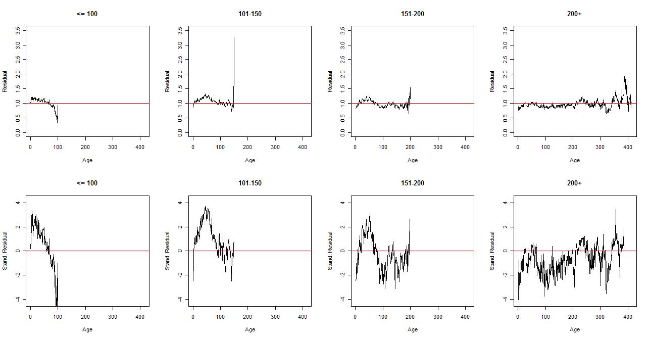
Running Variance
Rob Wilson defended the Yamal Substitution at CA in Feb 2006 on the grounds that the variance of the Polar Urals RCS chronology was “not stable through time” and that use of this version would therefore be “wrong”, whereas Yamal “at least had a roughly stable variance through time”.

Rob assessed the supposed variance instability using a 101-year windowed variance – a screening method likewise not mentioned in D’Arrigo et al 2006 nor, to my knowledge, elsewhere in the peerreviewedliterature. An obvious question is: how does the stability of the Polar Urals windowed variance compare to windowed variance on other RCS series that are in use? And does Yamal’s windowed variance show an “inner beauty” that is lacking in Polar Urals? The graphic below calculates windowed 101-year standard deviations for 13 Esper RCS chronologies (including Polar Urals) plus Briffa’s Yamal.


Figure . Running windowed-101 year standard deviation 850-1946 for 13 Esper RCS chronologies. Polar Urals in red; Briffa Yamal in black.

From 1100AD on, the Polar Urals chronology doesn’t seem particularly objectionable relative to the other Esper RCS chronologies. Its variance is elevated in the 15th century, but another Esper chronology has similar variance in the 12th century. Its variance is definitely elevated relative to other chronologies in the 11th century, a period in which there are only a few comparanda, most of which are in less severe conditions: the two strip bark foxtails and Tornetrask (Taimyr is presumably equally severe.)

Also shown in the above graphic is the corresponding graphic for Briffa’s Yamal series. Whatever points of reservation that Wilson may have regarding the Polar Urals RCS chronology would seem to apply even more with the Yamal chronology. Using Wilson’s rolling variance test, the variance of the Yamal chronology has been as high or higher than Polar Urals since AD1100 and has increased sharply in the 20th century when other chronologies have had stable variances. I am totally unable to discern any visual metric by which one could conclude that Yamal had a “roughly stable” variance in any sense that Polar Urals did not have as well. (Rob Wilson’s own comparison (see here used a different (his own) version of Urals RCS, where the rolling variance of the MWP is more elevated than in the version shown here using Esper’s RCS. However, Rob has also recently observed that he will rely on third party RCS chronologies and, in this case, Esper’s Polar Urals RCS would obviously qualify under that count.)

In respect to “rolling variance”, if anything, Yamal seems to have less “inner beauty” than Polar Urals.

Update: Kenneth Frisch in #207 below observes (see his code):

The results of these calculations indicate that the magnitude of the sd follows that of the mean and not that of the tree ring counts. Based on that explanatory evidence, I do not see where Rob Wilson’s sd windows would account for much inner beauty for the Yamal series or, likely, for any other RCS series (Polar Urals).

Yamal Already a “Standard”?
Another possible argument was raised by Ben Hale, supposedly drawing on realclimate: that Yamal was already “standard” prior to Briffa. This is totally untrue – Polar Urals was the type site for this region prior to Briffa 2000.

Briffa et al (Nature 1995), a paper discussed on many occasions here, used the Polar Urals site (Schweingruber dataset russ021) to argue that the 11th century was cold and, in particular, 1032 was the coldest year of the millennium. A few years later, more material from Polar Urals was crossdated (Schweingruber dataset russ176) and, when this crossdated material is combined with the previous material, a combined RCS ring width chronology yields an entirely different picture – a warm MWP. Such calculations were done both by Esper (in connection with Esper et al 2002) and for D’Arrigo et al 2006, but the resulting RCS reconstruction was never published nor, as noted previously, has the resulting RCS reconstruction ever appeared in print nor were the resulting RCS reconstructions placed in a digital archive in connection with either publication.

Instead of using and publishing the updated information from Polar Urals, the Yamal chronology was introduced in Briffa 2000 url, a survey article on worldwide dendro activities, in whichBriffa’s RCS Yamal chronology replaced the Polar Urals in his Figure 1. Rudimentary information like core counts was not provided. Briffa placed digital versions of these chronologies, including Yamal, online at his own website (not ITRDB). A composite of three Briffa chronologies (Yamal, Taimyr and Tornetrask) had been introduced in Osborn and Briffa (Science 1999), a less than one page letter. Despite the lack of any technical presentation and lack of any information on core counts, as noted elsewhere, this chronology was used in multiproxy study after another and was even separately illustrated in the IPCC AR4 Box 6.4 spaghetti graph.

Authors frequently purport to excuse the re-use of stereotyped proxies on the grounds that there are few millennium-length chronologies, a point made on occasion by Briffa himself. Thus, an updated millennium-length Polar Urals chronology should have been a welcome addition to the literature. But it never happened. Briffa’s failure to publish the updated Polar Urals RCS reconstruction has itself added to the bias within the archived information. Subsequent multiproxy collectors could claim that they had examined the “available” data and used what was “available”. And because Briffa never published the updated Polar Urals series, it was never “available”.

The Original Question
At this point, in the absence of any other explanation holding up, perhaps even critics can look squarely at the possibility that Yamal was preferred over Polar Urals because of its obvious exterior attributes. After all, Rosanne D’Arrigo told an astonished NAS panel: “you need to pick cherries if you want to make cherry pie”. Is that what happened here?

I looked at all possible origins of “inner beauty” that might justify why Yamal’s dance card is so full. None hold up. Polar Urals’ temperature correlations are as good or better than Yamal’s; Polar Urals is more “highly replicated” than Yamal since AD1100 with massively better replication in the 19th and 20th centuries; throughout most of the millennium (since approximately AD1100), Yamal’s windowed variance is as high or higher as Polar Urals and massively higher in the 20th century.

In summary, there is no compelling “inner beauty” that would require or even entitle an analyst to select Yamal over Polar Urals. Further, given the known sensitivity of important reconstructions to this decision, the choice should have been clearly articulated for third parties so that they could judge for themselves. Had this been done, IPCC reviewers would have been able to point to these caveats in their Review Comments; because it wasn’t done, IPCC Authors rejected valid Review Comments because, in effect, the IPCC Authors themselves had failed to disclose relevant information in their publications.

Proxy Inconsistency
Over and above the cherrypicking issue is the overriding issue of proxy inconsistency – a point made in our PNAS 2009 comment and again recently at Andy Revkin’s blog recently:

There are fundamental inconsistencies at the regional level as well, including key locations of California (bristlecones) and Siberia (Yamal), where other evidence is contradictory to Mann-Briffa approachs (e.g. Millar et al 2006 re California; Naurzbaev et al 2004 and Polar Urals re Siberia,) These were noted up in the N.A.S. panel report, but Briffa refused to include the references in I.P.C.C. AR4. Without such detailed regional reconciliations, it cannot be concluded that inconsistency is evidence of “regional” climate as opposed to inherent defects in the “proxies” themselves.

I repeat this point because without a reconciliation of such inconsistencies, without an ability to reconcile all the loose ends in regional climate, how can anyone in the field expect to carry out multiproxy studies.

Revkin Interviews Vaclav Smil

Andy Revkin invited me to his on-stage interview [instant replay here] of Vaclav Smil, a “historian of technical advances” and “intellectual agent provocateur”, at a public session of the “Quantum into Chaos Festival” (url) at the Perimeter Institute of Advanced Physics in Waterloo, Ontario near Toronto. Thus off to Waterloo late this morning and back to Toronto this afternoon. Andy said that Smil would be provocative and thought that I would enjoy his presentation. Smil has an interesting online speech from 2006 here in which he severely criticizes many popular “solutions” to present energy dilemmas as mere arm-waving.

There were about 120 or so people in the audience. Andy and Smil were onstage, Andy asked questions and Smil talked. As a blogger with an audience of my own, I thought that I would try to scoop Andy on his talk and thus here is my report on the afternoon. Continue reading

The NAS Panel and Polar Urals

Now that we know the abysmally low replication of the modern portion of Briffa’s Yamal chronology (something previously unknown to specialists), I’ve been backtracking through some earlier documents to see how this may have impacted past studies.

We’ve talked previously about how Briffa refused to provide measurement data to D’Arrigo et al 2006, resulting in them using Briffa’s Yamal chronology more or less blind.

For some inexplicable reason, their article worsens the situation by, in effect, conflating the two: they used the Yamal chronology, but, in the absence of Yamal core counts, used Polar Urals core counts! The NAS panel adopted this mishmash, also using the Yamal chronology together with Polar Urals core counts.
Continue reading