Trouet et al 2009 – More Info

On April 10, I was notified by NOAA that a little bit of data from Trouet was now online at NOAA WDCP. The archive is the absolute minimum; even Science would require them to archive this data if asked.

However, it is totally inadequate for replication.

However, every little bit of data helps and here’s a little progress report. It’s too bad that Esper the non-Archiver has taken an anti-archiving stance as the underlying idea of comparing the Scotland and Morocco proxies is fairly interesting. I’m still trying to understand why the authors regard this information as rebutting the MWP idea, as the proxies themselves seem to show a rather pronounced MWP/MCA.

First, the new data permits a more complete emulation of Trouet Figure S1, now that the Esper PDSI recon is available. For reference, below is the original Figure S1 with original caption.

Trouet Figure S1 Original Caption: Long-term winter proxy records from Europe. Comparison of the tree-ring based Morocco (S2) and speleothem based Scotland (S1) records with a documentary based estimate of September-June England-Wales precipitation (S10) and speleothem based estimate of winter temperature from the central Alps (S13) (A). Time series consist of 25-year averages, standardized over the common period (1075-1925). The Morocco PDSI record was inverted.

Next, here is my emulation of their Figure S1 using the speleothem version said by Andy Baker to be correct; the newly archived Esper PDSI information; my manual transcription of data from Lamb 1965; and archived Mangini information. In each case, I’ve used 50-year averages and then scaled the resulting series over 1075-1925 as in the Trouet caption, orienting the series to match the Trouet figure. As noted previously, 50-year averages match. Three of four emulations match very closely: the oddball is the Scotland speleothem, where, as noted before, Trouet has almost certainly used the detrended version, said by Andy Baker to be an incorrect version. (Andy Baker said that Trouet used the non-detrended version but I don’t think that his understanding is correct; I’ve emailed him about this.)

Figure 2. My emulation of Trouet Figure S1.

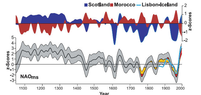
Moving along a little, here is Trouet Figure 1 from the main article. The term “30-year cubic spline” may not be familiar to statisticians and scientists from Off the Island; I think that I can explain what this means in Team dialect and will do so if necessary. Note that the two series are oriented oppositely in this plot (while the MWP has a common orientation in SI Figure 1.)


Original Caption to Trouet Fig. 1. Proxy-derived long-term NAO reconstruction. (Top) Reconstructed winter precipitation for Scotland and February-to-June Palmer Drought Severity Index (29) for Morocco. Records were normalized over the common period (1049–1995) and smoothed with the use of a 30-year cubic spline. (Bottom) Winter NAO reconstruction NAOms (black curve) is the difference of the Scotland and Morocco records. The gray area is the estimated uncertainty; yellow and red areas are the 10 and 33% highest and lowest values since 1700. The blue line represents the 30-year smoothed Lisbon-Iceland instrumental NAO index series (11).

Most CA readers hate all the smoothing of data that’s infected so many Team articles and presentations, including Trouet et al. For comparison, in the next figure, I’ve plotted raw versions of the two series in question – the Esper PDSI recon (however it was made) and the Baker non-detrended speleo, said to the preferred version, though, as noted above, unlikely to be the version used in Trouet.

Examining the “raw” versions of the data, here are my first few comments.

1. The “correct” non-detrended Scottish speleo data – whatever it shows – definitely shows a “warm” MWP on the scale of the late 20th century. The ability of the proxy to measure warm climates looks severely limited by the fact that it has a zero minimum and is bumping against the zero minimum in the MWP.

2. The eye can certainly be teased into comparing the two series. And in fairness to this perception, both series had been postulated to be connected to the NAO in independent articles (Proctor et al 2000, 2002) and Esper et al 2007, before the present joint venture article. IF both series are NAO proxies, then the big downspikes should align. Given the precision of tree ring dating, I think that there would be an excellent case for using the tree ring data to align the speleo data with its much looser dating control. I’m not exactly sure how one would express this methodology in objective statistical terms, but intuitively it makes sense to me. Perhaps Roman or UC or Hu have ideas on this.

3. Esper’s PDSI reconstruction has all sorts of ad hoc splicing, selecting and re-scaling, but it’s not possible analyse its impact without the Esper measurement data, which is under lock and key.

Reblog this post [with Zemanta]

Ammann’s April Fool’s Joke Part 2

About 2 weeks ago, I observed that the PR (Paleoclimate Reconstruction) Challengers, stung by various challenges to the non-transparency of their data and methods, had promised that, by April 2009, they would, among other things, make a website containing:

– Collection of reconstruction codes, documentation, and related data.

Interestingly, on April Fool’s Day itself, NOAA released a webpage, which I presume is supposed to be the April 2009 deliverable.

At first blush, it looks like something new.

However, many temperature reconstructions had already been archived. That’s how you make the spaghetti graphs. The PR issue has always been the availability of underlying data and reconstruction codes – the things that the PR Challengers promised to deliver by April 2009.

The “new” data is simply a collation of the reconstructions already listed on the NOAA webpage. The various textfiles here contain references to the prior WDCP page. For example, the new page ftp://ftp.ncdc.noaa.gov/pub/data/paleo/reconstructions/pcn/textfiles/biondi1999.txt cross-references ftp://ftp.ncdc.noaa.gov/pub/data/paleo/treering/reconstructions/northamerica/usa/idaho/idaho-temperature.txt.

Bizarrely, NOAA itself already had catalogued temperature reconstructions, listed on its webpage here (predecessor page here)

So the deliverable is nothing except a collation of temperature reconstructions already listed on NOAA’s reconstruction webpage, together with some elementary metadata.

No proxy data. No source code. No documentation beyond the most trivial metadata.

For me, the collation has no utility. I already have read scripts for about 50% of the reconstructions, with annotations that are more helpful reminders about what’s in the data than the present trivial metadata.

I’m not sure who’s going to use this collation or what PR problem it’s supposed to solve. I wonder how much NOAA paid for this (without even considering staff time). I would sure liked to have had the opportunity to bid on the contract.

Esper in Morocco

The other series in Trouet that contributes to their NAO reconstruction is the Morocco chronology from Esper the non-Archiver. In the Scotland speleo series, we observed an awkward detrending step prior to the NAO reconstruction. In the Morocco series, there proves to be some awkward splices: a splice of two different series versions at a hinge point of AD1300; and the use of different normalization curves before and after AD1600.

The net effect of these splices is impossible to assess on the present record as none of Esper’s measurement data is archived and, in detail, his methods remain obscure. Nonetheless, evidence is presented here to indicate that these splices result in a substantial detrending relative to an RCS chronology based on the 40% of the data available from prior archiving by Stockton.

Unfortunately, the pending “data” contribution from Trouet et al is limited to the NAO reconstruction and the spliced Esper PDSI reconstruction, neither of which suffice to permit proper assessment of the article. Esper the non-Archiver has not archived his underlying Morocco measurement data.

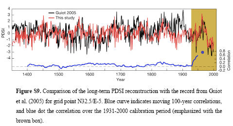
Let’s start with the Esper drought (PDSI) reconstruction. The same series is illustrated in multiple versions (maybe the referees thought that this was different information, but it’s all the same.) In each case, there is a closing a downtick representing seemingly unprecedented drought.

or here
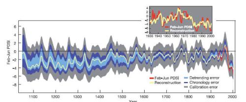
or here (being compared to another NAO reconstruction with which it has zero correlation):

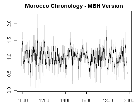
Alert CA readers may recall that a Morocco chronology (morc014) was a component of MBH99 (back to AD1000), one that was re-used in Juckes et al 2007 (non-inverted) and I’ve compared this data as well (see the graphic below). If you squint back and forth, you can see considerable correspondence between the decadal peaks and downticks, but the MBH/Juckes version looks like nothing more than noise in terms of MWP-LIA-Modern variability (and indeed, white noise performs just as well as a bristlecone condiment).

Any dendros reading this post will observe that the chronologies used in the Mann-Juckes recon couldn’t have been “conservatively standardized”. While one would have thought that left and right had no natural orientation in dendochronology (which has a hard enough time deciding whether a series should be oriented up or down), “conservatively” in this context means something like RCS standardization, where one age model is determined for the data set and used to standardize all the series (as core by core standardization with short splines will yield things that look like the MBH version.)

As noted above, Esper hasn’t archived his measurements, so let’s look at the very large (40%) sample of measurement data that is archived and carry out our own RCS analysis.

Esper 2007: Tree-ring data used in this study include ~64,000 annual ring width measurements from Cedrus atlantica trees sampled in 1985 [Glueck and Stockton, 2001], and a newer collection of ~100,000 measurements sampled in 2002.

First, retrieve the data – the following script picks the data up from WDCP and organizes it into a data frame for easier analysis – columns being core ID, year, age and ring-width. My retrieval function make.rwl is a very old function for me (~2003); I’d write it more cleanly now, but it works – here downloading 63,734 measurements from 7 Stockton sites. The total number of measurements match the number reported above in Esper et al 2007 and the sites are listed in the Esper SI so this is apples and apples. The newer Esper data supposedly focuses more on older trees, but without any data, it’s impossible to comment on the reliability of this statement.

id=c(paste(“morc00″,1:3,sep=””), paste(“morc0″,11:14,sep=””))
source(“http://data.climateaudit.org/scripts/utilities.treering.txt”) #use make.rwl
Data=NULL
for(i in 1:length(id)) {
tree=try(make.rwl(id[i]))
Data=rbind(Data,tree)
}
dim(Data)
#[1] 63734 4

In this example, plot of average ring width against age shows a very nice negative exponential form, as shown below:

The above plot was given by:

tree=Data #I’m used to using tree as a name for this sort of data
aging=tapply(tree$rw,tree$age,mean)
fm=nls(rw ~ A+B*exp(-C*age),data = tree,
start = list( A=mean(tree$rw,na.rm=T)/4,B = mean(tree$rw,na.rm=T), C= .01 ),
alg = “default”, trace = TRUE,control=nls.control(maxiter=200, tol=1e-05, minFactor=1e-10));
B=fm$coef;round(B,5) #546.76899 1501.98114 0.01079
fit.fm< – B[1]+B[2]*exp(-B[3]*(1:max(tree$age)) )
par(mar=c(4,4,2,1))
plot(as.numeric(names(aging)),aging,type="l",ylab="Ring Width",main="Morocco RW by Age",col="grey50",xlab="Age")
lines(1:max(tree$age),fit.fm)

Next we’ll calculate an RCS- chronology which, as I understand it, consists of standardizing all ring widths by fitting one growth curve. I’ve used my own algorithm here, which is based on careful study.

source(“http://data.climateaudit.org/scripts/treeconfig.functions.txt&#8221;)
test= RCS.chronology(tree,method=”nls”)

I’ve occasionally posted RCS emulations in the past, sometimes provoking screeches from dendros that I’ve done something or other “WRONG”, but I was unsuccessful in eliciting any data sets where there are both archived measurement data and RCS chronologies and, to my knowledge, none of the public dendro software uses these methods contains an RCS module. The underlying math is pretty simple – here I’ve fit one age curve to the data and standardized on that basis. This yields the following RCS chronology – one which looks like neither the MBH version nor the Esper version, though, once again, if you squint back and forth, you can match the decadal variations.

What accounts for this difference? Well, Esper has more recent data that yields a downtick at the end of his series. Add a downtick to the above chronology and we’re still left with a conundrum.

Esper has considerable supplementary material online here that may have some clues.

First, Esper describes the elimination of about 34,000 measurements as follows:

Common variance between the nearby site chronologies from Tiz, Col, Tou, and Jaf supported combination of the old growth data into a merged dataset TCTJ integrating 326 tree-ring series consisting of ~134,000 annual width measurements.

On another occasion, Esper stated:

However as we mentioned earlier on the subject of biological growth populations, this does not mean that one could not improve a chronology by reducing the number of series used if the purpose of removing samples is to enhance a desired signal. The ability to pick and choose which samples to use is an advantage unique to dendroclimatology.

One hopes that this was not the justification for deleting 34,000 measurements.

Second, Esper used a different age-curve for data prior to AD1300 and after AD1300. This is described as follows:

the combined Norm-RCS record is represented by Norm back to 1300 and by RCS Old prior to this year.

Esper purports to justify this splice by observing a high correlation between these versions. Needless to say, a high correlation can co-exist with a drifting apart of the two versions and this would need to be examined in detail.

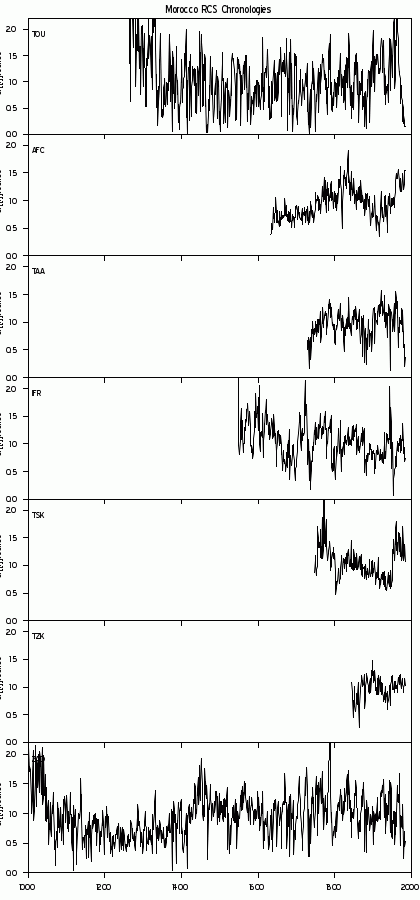
Thirdly, although one of the purposes of RCS methods is to have uniform age curves, Esper uses a different age curve for “Old” data (152 tree-ring series before AD 1600 and 174 series after AD 1600, respectively), as shown below:
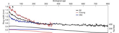
It seems fairly clear that this use of different normalization curves before and after AD1600 results in a considerable de-trending of the RCS chronology. How is this justified?

Analysis of the RCS method applied to all TCTJ data indicated that resulting chronologies contain increasing long-term trends that are possibly exaggerated by the inclusion of measurement series from younger trees. This potential bias has been assessed by splitting the TCTJ data into Young and Old sub-samples, integrating 152 tree-ring series less than AD 1600 and 174 series greater than AD 1600, respectively. Alignment of these sub-samples by cambial age revealed substantial differences in initial growth rates and age trends (Figure S4). The Young data contain much wider rings (initially about 1.6 mm) and a steeper age trend than the Old data (first rings about 1.1 mm). …

These differences might to some extent arise from the tendency of greater pith offset (PO) – which is the difference in years between the innermost ring on a core sample and the true center or pith of a tree at sampling height – in larger trees [Esper et al., 2006]. In other words, there is a tendency that more innermost tree-rings were missed on core samples from old trees than on samples from young trees. The key reason for this tendency is the sheer size of Moroccan cedar trees, with individuals frequently exceeding diameters of 4-5 m at breast height. As a consequence, differently old tree-rings are related to each other within the RCS procedure [Esper et al., 2003a]. This is particularly important as the young trees, with greater growth values cover only the recent end of the chronology. And as such, they may impart a bias towards a positive trend in recent times.

This last sentence should be quite worrying to dendros. In this particular case, Esper, expecting the data to go down in the post-1980 period, identified a potential bias in young trees relative to old trees. But what of the far more common case where increasing ring widths are expected? How often do we see dendros (Esper himself for that matter) assessing the data against a “bias towards a positive trend in recent times”. Doesn’t seem to happen.

Update: I’ve run separate RCS by each site. The average RW at TZK is about 6 times the width at Col du Zad. The upward trend in the overall RCS plot is therefore mainly due to inhomogeneity in site location, with an increasing mix of high growth sites. This seems like a far more plausible stratification than Esper’s peculiar attempt to stratify Young and Old trees.

Reference:
Jan Esper, David Frank, Ulf Buentgen, Anne Verstege, Juerg Luterbacher, and Elena Xoplaki, 2007. Long-term drought severity variations in MoroccoGRL 2007 url

De-Trending in Scotland

The two proxies that carry the water in the Trouet NAO reconstruction are the Baker speleothem in Scotland and Esper’s tree ring chronology in Morocco.

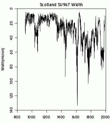
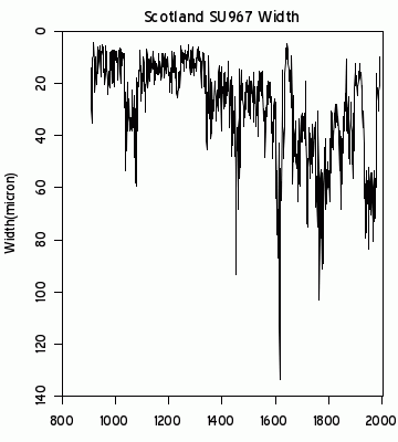
The briefest examination of the Scotland speleothem shows that the version used in Trouet et al had been previously adjusted through detrending from the MWP to the present. In the original article (Proctor et al 2000), this is attributed to particularities of the individual stalagmite, but, since only one stalagmite is presented, I don’t see how one can place any confidence on this conclusion. And, if you need to remove the trend from the MWP to the present from your proxy, then I don’t see how you can use this proxy to draw to conclusions on relative MWP-modern levels.

For reference, the following graphic shows the Trouet version:

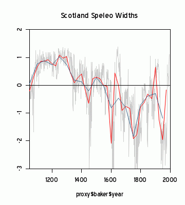
As Andy Baker explains in his article and in a CA comment, speleo widths are believed to be narrower in warm and wet periods and wider in cold and dry periods (with temperature and precipitation not being independent due to NAO). Based on this, I’ve plotted the original data in an inverted sense (narrower at the top) in the top left. I’ve plotted the full speleothem (Trouet cuts off at AD1075 or so). They transform the data to z-scores even though the data is highly non-normal. The z=score distribution is truncated at an sd of about 1, corresponding to the minimum width of about 0. Also shown are 25-year and 50-year binned averages. As noted before, although Trouet et al say that they used 25-year averages, they actually used 50-year averages.


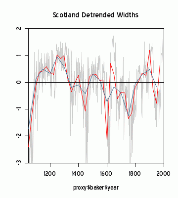
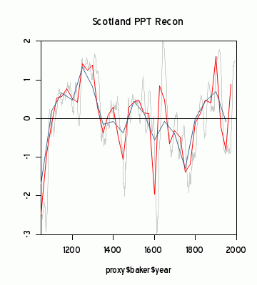
Figure 1. Versions of SU967 Speleothem.

The bottom left shows the same plot for the “detrended” widths, while the bottom right shows the same plot for the “precipitation reconstruction” which is a re-scaling (linear transformation) of the detrended width series. This is the version that is carried forward into Trouet. The “detrending” (also called “normalisation”) is described in Proctor et al 2000 as follows:

Personally, I find this justification underwhelming. The adjustment leads to important reversals of medieval-modern relationships – all in the direction of enhancing 20th century levels relative to 11th century levels. Even if the adjustment subsequently proves justified (and there are circumstances in which it could come onside), you can’t assign any confidence to any product of this data set without assessing potential errors in the detrending. Unfortunately, Trouet et al neglect this error source:

These individual error terms include (i) dating uncertainties of the speleothem record, (ii) chronology error of the tree-ring record, and (iii) calibration error of the residual record NAO_ms.

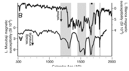
Actually the non-detrended Scottish speleothem record reminded me of the Polissar glacier discharge proxies from Venezuela of all places, as shown below (Discussed a couple of years ago at CA), both showing transitions from ‘MCA’ to LIA around 1250-1300. I submit that this is no less “remarkably similar” than any of the Team comparanda. This is not actually inconsistent with the actual language of Trouet et al where a global reorganization of wind fields at the ‘MCA’-LIA transition is posited.


Reference:
Proctor et al 2000: http://www.barlang.hu/pages/science/angol/CD2000_815.pdf

Data Archiving for Trouet-Esper

Trouet et al was released on April 2, 2009 with an SI that did not include any data. Discussion began here on April 3 in the comments here and later that day I posted on it here observing:

Unfortunately, the authors failed to provide any digital data citations (see for example AGU policies on this, though AGU journals don’t require climate scientists – and perhaps others – to comply with these policies), though they provide references to dead tree literature from which the data provenance for 3 of the 4 series can be plausibly surmised. The “tree-based Morocco” data set is from Esper the non-Archiver, previously published in GRL without archiving any data. (Esper the non-Archiver flouted AGU policies requiring use of archived data – not that AGU journals bother enforcing what on paper is an excellent policy.)

On April 5, after coauthor Baker commented briefly commented at CA, I asked him for digital versions of the NAO series and Morocco chronologies used in the article. He notified me today that Trouet had already submitted “the data” to WDCP on Friday and therefore did not send me anything.

I hope (against hope) that Trouet has archived more than just the bare minimum of their NAO reconstruction. Here are other things that one needs to examine this article.

In addition to the unarchived Morocco chronology, they illustrate other series that are not in the public domain: e.g. an Iceland ocean sediment series; also, in some cases, they cite articles that have many series (e.g. Lund et al 2006) and do not specify which series was used, leaving the reader to try to guess what they did. I have no expectation of proper data citations (e.g. in compliance with unenforced AGU policies, but it would be nice to be surprised for once.)

The Esper Morocco chronology is derived from unarchived measurement data, published in Esper et al 2007 in GRL (where as noted in a prior post, Esper flouted AGU policies on data archiving and the referees and editors didn’t care – not that they bother enforcing the policy against anyone). Esper’s chronology incorporates Stockton data that is archived, so Esper is not reluctant to use measurement data archived by others; he’s just reluctant to reciprocate. I’ve done a quick RCS chronology on the ~64,000 measurement data on archive from Stockton up to the mid-1980s and get a different looking chronology than Esper. You cam get different chronologies using different methods, so the measurement data is an essential part of any tree ring-based article, as Esper’s friend, Rob Wilson, will confirm. I hope (against hope) that Trouet has finally archived the Morocco measurement data.

In any event, I’ll see whether the archive is complete and report on my progress.

Ryan O on the Cloudmasked Data

Following excellent notes transferred from a comment by Ryan O, who has been doing excellent analyses of the Steigian swamp. Continue reading →

Jeff on Steig RegEM

Jeff has made some progress on the basis that PC was applied to the AVHRR data before RegEM. See a good post here .

This is obviously inconsistent with claims at realclimate.org by Gavin Schmidt and Eric Steig, but we’ve known for a while that their explanations are not accurate.

This is a different exercise from assessing whether the method makes any sense and an effort that is required only because of inaccurate documentation, lack of data and continued obfuscation by PR Challengers Schmidt and Steig.

Esper's April Fool's Joke

Esper the non-Archiver is Trouet’s supervisor (see url.), so I’ve taken the liberty here of ascribing this clever April Fool’s prank to Esper, though undoubtedly Trouet deserves some credit for her role in pulling off the prank.

In a recent post, I alluded to the point that the England precipitation index shown in the Trouet Esper graphic below is derived from Figure 4 of Lamb 1965.

The idea that Lamb’s reconstruction should be held out as a key element in their disproof of the Medieval Warm Period is such a pretty prank that it really deserves to be savored a little more than we’ve done so far. It’s almost as good as prank as Mann using Sherwood Idso’s strip bark results to disprove that MWP. Maybe it’s a better prank since it uses a variation of the IPCC 1990 graphic itself: the link between the IPCC graphic and the Lamb-Esper precipitation series being readily seen in the following excerpt from a Lamb graphic – the rounded version is carried forward into the well-known IPCC 1990 graphic while the more angular version is carried forward into the Esper-Trouet Figure (compare to the cyan line in Trouet-Esper graphic):

Anyway, today I thought it would be interesting to report on exactly how Lamb derived his estimate of winter precipitation, as readers should take care to be aware of exactly what’s in Lamb’s winter precipitation estimate so that they can better protect themselves against pranksters like Esper.

Lamb’s original Table II excerpt for rainfall is shown below – the first column is annual, 2nd is high summer (July-August) and the 3rd is the rest of the year (Sept-June), all expressed as percentages of 1916-1950 values.

The high summer rainfall is calculated through a regression relationship with the “Summer Wetness Index” of Lamb and Johnson, 1961 (I don’t know how this Summer Wetness Index was calculated and have no plans at present to investigage this rabbit hole further).

The regression equation for decade values of July and August rainfall (as % of the 1916-1950 average) over England and Wales (R_JA) on the summer wetness index value (W) is: R_JA = 6.52W + 29.1. The standard error of the resulting percentage figure appears to be ± 4.01. (p. 26)

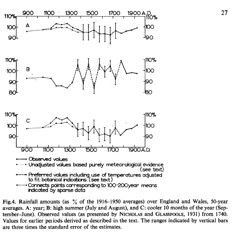
Next the annual rainfall was calculated through a 2nd regression relationship – this time with the famous Lamb temperature reconstruction (which is why the shape ends up being so familiar).

The estimates of average yearly rainfall in Table II and Fig.4 are derived from the yearly mean temperatures given, and from the winter temperatures adjusted to be at their mildest in the medieval warm epoch the equal of the present century, using the appropriate regression equations[2] …

Footnote 2: The regression equation for decade values of average yearly rainfall in England and Wales (Ry) as % of the 1916-1950 average rain on average yearly temperature Ty is: Ry = 9.80Ty + 6.2. The standard error of the percentage estimates so derived appears to be 4.65.

Thus, Lamb’s estimate of annual rainfall is a linear re-scaling of the famous temperature series. (BTW the IPCC 1990 is a little different than the Lamb 1965 version and appears to be taken from a slightly different version in Lamb 1967, as discussed in a post on an earlier occasion.)

Next the Sept-June rainfall is estimated as the difference between the two values:

Finally, the rainfall averages in Table II for the 10-month period that excludes the high summer, were given by the differences between the amounts of rain implied by the other two columns.(page 33)

The reason why the Lamb-(Esper) winter precipitation estimate has the same shape as the famous annual temperature series is that the summer wetness index does not have a lot of “low frequency” variability relative to the annual temperature series, and thus the famous shape carries through to the winter index.

Somewhat inconsistently, footnote 2 on page 33 reports a third regression equation relating Sept-June rainfall to temperature as below (the running text appears to indicate that it was calculated by difference; I haven’t tried to verify which is the case as it doesn’t matter for present purposes):

The corresponding regression equation for values of rainfall over the 10 months September- June (R10) on winter temperature is: R10 = 7.81 T_DJF + 66.6. The standard error of these estimates appears to be 4.29.

As you can see from Table II, there aren’t a lot of degrees of freedom in any of these regression equations.

Here again, Esper has again pulled a very clever prank as he’s smoothed all his data into 50-year bins as well, so that no one can complain about about overly coarse data in Lamb 1965. Esper has done an additional tease by saying that they used 25 year bins even though the merry prankster used 50 year bins as shown in my earlier post.

All in all, even CA readers must grudgingly respect both Esper and Science for pulling off such an inventive and witty April Fool’s prank.

Two Quotations

Here are two quotes. The first is from Trouet et al 2009:

The increased pressure difference between the Azores High (+3 hPa) and the Icelandic Low (–5 hPa) during positive NAO phases results in enhanced zonal flow, with stronger westerlies transporting warm air to the European continent. The axis of maximum moisture transport and the preferred stormtrack extend further to the north and east during positive NAO phases when the Azores High is strengthened, resulting in wetter winters over northwestern Europe (50-to-200–mm positive anomalies per season) and decreased precipitation over southern Europe and northwestern Africa (50-to-100–mm negative anomalies per season).

The next quotation is not:

Judged by the implied shift of the upper westerlies, the main depression tracks and the zone of low pressure associated with them (the “Iceland low”) should have had, in the period 1000-1300, an average position 1-3 ° north of the modern normal (1900-1939 average) position– a displacement that probably implies less ice on the Arctic seas, because a northward progression by almost this amount between 1800 and 1940 went hand in hand with a roughly equal retreat of the ice…

The [MCA] appears as one of dry summers, i.e., an oceanic, summer anticyclonic type of regime. In the subsequent cold epoch,… the summers have contributed a more than proportionate share of the year’s rain, whereas the winters became relatively dry.

The exercise for today is 1) to identify the source of the second quotation [PLEASE DO NOT GOOGLE as anyone can google things and you immediately encounter a PPT that reveals the source] and 2) explain exactly how the Trouet et al 2009 explanation overturns (or even differs) from the explanation in the other article.

Trouet et al 2009: “Scuppering the Deniers”

Trouet et al (2009), Persistent Positive North Atlantic Oscillation Mode Dominated the Medieval Climate Anomaly, published in Reader’s Digest Science a few days ago. Esper the non-Archiver is a co-author. New Scientist breathlessly reported :

Europe basked in unusually warm weather in medieval times, but why has been open to debate. Now the natural climate mechanism that caused the mild spell seems to have been pinpointed.

The finding is significant today because, according to Valerie Trouet at the Swiss Federal Institute for Forest, Snow, and Landscape Research in Birmensdorf, the mechanism that caused the warm spell in Europe – and meant wine could be produced in England as it is now – cannot explain current warming. It means the medieval warm period was mainly a regional phenomenon caused by altered heat distribution rather than a global phenomenon.

The finding scuppers one of the favourite arguments of climate-change deniers. If Europe had temperature increases before we started emitting large amounts of greenhouse gases, their argument goes, then maybe the current global warming isn’t caused by humans, either.

Michael Mann told the New Scientist that the new results may imply that the situation is even worse than we thought.

If one actually reads the article, the word “regional” only occurs once

The North Atlantic Oscillation (NAO) … has a substantial influence on marine and terrestrial ecosystems and regional socio-economic activity

The word “phenomenon” is not used anywhere. Nor are the words “altered” or “heat distribution”. If New Scientist is correctly reporting her statements, I did not locate anything in the article that specifically supports the reported oral summary of the conclusions. Indeed, the following sentence seems to suggest the exact opposite – that the transition from the “MCA” to the Little Ice Age was “globally contemporaneous” and, in language reminiscent of Hubert Lamb, that this was due to “a notable and persistent reorganization of large-scale oceanic and atmospheric circulation patterns”:

The relaxation from this particular ocean-atmosphere state into the LIA appears to be globally contemporaneous and suggests a notable and persistent reorganization of large-scale oceanic and atmospheric circulation patterns.

I take no position in the present post on whether the MCA was or wasn’t global – I’m merely observing that the article itself does not draw the conclusion that was reported in the aftermarket promotion. Penny mining stock press releases are not permitted to go beyond the information in their prospectuses or qualifying reports and it always surprises me to see climate scientists issue press releases that promote well beyond the four corners of what was approved for publication.

In a quick read, I spotted a number of issues that are of interest, not all of which will be covered in today’s note. On another occasion, I’ll try to connect the present analyses of NAO and the Atlantic meridional overturning circulation to what Hubert Lamb and William Gray said on these topics respectively (please save such comments for another day.)

Today I’ll post some notes on the provenance of the data. Their NAO reconstruction is based on a comparison of highly smoothed Scottish speleothem bandwidth data to a Morocco tree ring chronology by Esper the non-Archiver. They also refer to an England-Wales (EW) documentary precipitation reconstruction, which surprisingly proved to be from Lamb (1965) and an Alps temperature reconstruction by Mangini – the one that Gavin Schmidt complained about when Loehle used it. Scottish speleothem data was used in Mann 2008 as a temperature proxy, while an earlier version of the Morocco tree ring chronologies was used in MBH98, MBH99 and Juckes 2007, again as a temperature proxy.

Their Figure S1 illustrating their 4 money proxies is shown below. Given that the article is said to refute MWP concepts in some sense, it’s a little surprising that none of the underlying data in their illustration is particularly HS-shaped; on the contrary, these data sets all seem to have a medieval “anomaly” as pronounced as the modern anomaly.


Trouet Figure S1 Original Caption: Long-term winter proxy records from Europe. Comparison of the tree-ring based Morocco (S2) and speleothem based Scotland (S1) records with a documentary based estimate of September-June England-Wales precipitation (S10) and speleothem based estimate of winter temperature from the central Alps (S13) (A). Time series consist of 25-year averages, standardized over the common period (1075-1925). The Morocco PDSI record was inverted.

Unfortunately, the authors failed to provide any digital data citations (see for example AGU policies on this, though AGU journals don’t require climate scientists – and perhaps others – to comply with these policies), though they provide references to dead tree literature from which the data provenance for 3 of the 4 series can be plausibly surmised. The “tree-based Morocco” data set is from Esper the non-Archiver, previously published in GRL without archiving any data. (Esper the non-Archiver flouted AGU policies requiring use of archived data – not that AGU journals bother enforcing what on paper is an excellent policy.)

The Scotland speleothem series is attributed to Proctor et al 2000, for which data is archived at NCDC. In the right panel below, I show rescaled versions of the archived Proctor precipitaiton reconstruction, including original data raw (blue), 25 year average (red) and 50 year average (navy blue). Although Trouet et al stated that “Time series consist of 25-year averages, standardized over the common period (1075-1925)”, this appears to be untrue as their Figure S1 does not match a 25-year average, but does match a 50-year average. This would obviously reduce the degrees of freedom even further from the already substantial reduction and the effect of this, if any, needs to be checked.


Figre 2. Left – Trouet Figure S1; right – Proctor ppt recon from speleothem: blue – as archived; red – 25 year average; navy blue – 50 year average,

The cyan series September-June England-Wales precipitation in Trouet Figure S1 has a very familiar looking shape. S10 is Lamb 1965; the shape of this figure may remind keen-eyed readers of the famous IPCC temperature curve (derived from Lamb) showing the MWP. See discussion at CA here which has many relevant figures. Here is Lamb 1965 Figure 4 showing the precipitation reconstruction, which is related to the temperature reconstruction (I’ll try to get to this on another occasion. For interested readers, I’ve placed Lamb 1965 online – see below – it has many comments about wind circulation relevant to the present discussion. As discussed on another occasion, IPCC AR4 sneered at Lamb’s work: “Lamb’s analyses also predate any formal statistical calibration of much of the evidence he considered.” I don’t want readers to spend any time debating the merit or lack of merit of the IPCC criticis, (which one disregarded reviewer took some exception to). What’s intriguing in the present context is that Lamb’s reconstruction is used to scale the Scottish speleothem record, perhaps a surprising calibration method under the circumstances.

For the PSR analysis in this work, the Scotland speleothem record was transformed into precipitation (as fraction of modern climatology) using Lamb’s documentary evidence-based estimate of a 13% MCA-to-LIA reduction in September-June England-Wales rainfall (S10).


Lamb 1965 Figure 4 showing rainfall reconstruction. Sept-June precipitation is in the bottom panel.

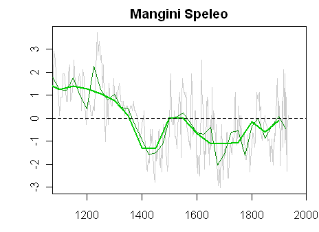
The green series in Trouet Figure S1 is from Mangini’s temperature reconstruction from speleothems – again this appears to be the 50-year average, rather than the 25-year average as shown below using original data.


Figure 3. Re-scaled Mangini temperature reconstruction.

We’ve discussed this series a couple of times in the past. Gavin Schmidt excoriated Loehle’s use of this data here (See CA discussion here, on the basis that “no validation of this temperature record has been given” and that it had “been given a unique negative correlation to temperature.”

Unfortunately, no validation of this temperature record has been given… However, only one terrestrial d18O record is used by Loehle (#9 Spannagel), and this has been given a unique negative correlation to temperature…

Trouet calibrate the Mangini speleothem against a documentary series (I haven’t looked at this calibration yet) and arrive at the same “unique negative” orientation as the one that Schmidt complained about in Loehle’s usage. The difference in scale noted below would not affect the z-score plot shown here.

For Alps temperature, the smoothed (25-year running mean) Spannagel (S13) record was calibrated using linear regression against smoothed area-average (6-14E, 46-48N) December-February temperature from a documentary evidence-based data set (S14, S15) over the period 1525-1903. The correlation between these records is 0.69, with both time series showing four distinct peaks (see Fig. 4 in (S13)) over the calibration period. No rescaling was applied for this reconstruction. The resulting reconstruction gives an MCA-to-LIA winter temperature decrease in the Alps of approximately 0.4° C.

The article calculates many statistics and I’ll review some of these calculations if and when the relevant data is archived. The data has been hugely smoothed – a practice abhorred by most working statisticians (See Matt Briggs on this)- and I’d be surprised if the significance calculations hold up, but we’ll see.

References:
Trouet, V, Esper J, Graham NE, Baker A, Scourse JD, Frank DC (2009) Persistent positive North Atlantic Oscillation mode dominated the Medieval Climate Anomaly. Science 324, 78-80. (pdf)
SI
Lamb 1965 url