Lucia has written an interesting post – see here, continuing the effort to figure out the Santer brainteaser.
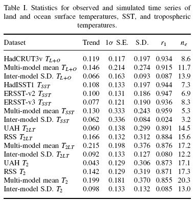
I can shed a little more light (I think) on what Santer’s “S.D” is in operational terms. I was able to replicate Santer’s Table III values using the line item from Table 1 entitled “Inter-model_S.D._T2LT” which is shown in column 1 (“Trend”) as being 0.092. So this number – whatever it is – is the one that is used as the other component of the denominator in his t-test.
Santer did not archive the 49 time series as used and thus far has not responded to my request for this data.
The caption to Santer Table 1 says:
The multimodel mean and inter-model standard deviation were calculated using the ensemble-mean values of the time series statistics for the 19 models [see Equations (7)–(9)].
Now there is a bit of helpful information in Douglass Table 1, which provides ensemble-mean values for 22 models – I haven’t checked to see which models are different. Douglass Table 1 provides model ensemble trends by altitude, but not weighted according to T2LT weights. John Christy sent me weights by email and I calculated T2LT trends according to these weights as follows:
douglass=read.table(“http://data.climateaudit.org/data/models/douglass.dat”,header=TRUE,sep=”\t”)
name1=names(douglass)[4:15]
alt=as.numeric(substr(name1,2,nchar(name1)))
douglass[,3:15]=douglass[,3:15]/1000 #converts to deg C/decadechristy.weights= c(0.1426, 0.0706, 0.1498, 0.1894, 0.1548, 0.1382, 0.1035,
0.0477, 0.0167, 0.0067, -0.0016, -0.0179) ##CHRISTY WEIGHTS email Apr 30 2008
names(christy.weights)=alt
douglass$trend_LT= apply(douglass[,c(3,5:15)],1,function(x) weighted.mean(x,christy.weights) );
douglass$trend_LT
# 1] 0.176 0.131 0.427 0.144 0.268 0.212 0.141 0.093 0.175 0.245 0.337
sd(douglass$trend_LT) #[1] 0.0913
The standard deviation of 0.0913 from this calculation compares nicely with the value of 0.092 in Santer Table 1 for UAH_T2LT, so it looks like this is apples and apples.
In the subsequent t-calculation for Table III, Santer (like Douglass) divides this number by sqrt(M-1), where M is the number of models, yielding a value of 0.02152. So Santer, like Douglass, in effect proceeds on the basis that the 95% CI envelope for the ensemble mean trend is 0.171- 0.257 deg C/decade. The majority of individual models are above 0.171 deg C/decade.
Now here’s a quick simulation that implements what I believe to be a fairly reasonable interpretation of what should be done (considering the sorts of points that beaker and others have made).
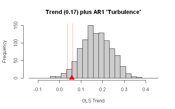
First I assumed that the ensemble mean was the true trend; I centered everything at their midpoints and then calculated residuals from the observed values. I then did an arima AR1 fit to the residuals getting an AR1 coefficient of 0.89 – a little higher than with a better fit and a sd of a little over 0.14 (deg C/decade). I then did 1000 simulations in which I generated AR1 “noise” with parameters of AR1= 0.89 and sd=0.141, added the AR1 noise to the ensemble mean trend ( a straight line), calculated the OLS trend for each run and made a histogram as shown below, also showing the observed OLS trend as a red triangle and the 2.5% and 5% percentiles. The observed OLS trend is outside both percentiles.

Histogram of OLS Trends adding AR1 noise (AR1=0.89, sd=0.141) to ensemble mean trend
Next, I did the same thing assuming a trend of 0.17 (the lower limit of CI interval on ensemble means) and a level that picks up a few important individual models. In this case, the observed OLS trend is outside the 5% percentile, but inside the 2.5 % percentile.
Suppose that Santer now says in Mannian tones: you are “wrong”!!!! You haven’t allowed for uncertainty in the observations. Haven’t you read about the uncertainty attached to an OLS trend in the presence of autocorrelation?
But haven’t we already dealt with that by generating this type of “noise” in our simulations. Aside from the big problem between RSS and UAH, we know what the observed OLS trend and the AR1-type uncertainty does not enter into this calculation. We compare one OLS trend to the distribution of OLS trends generated by our simulation.
And BTW, I sure don’t get why this has to get to a 5% or even 2.5% level of significance before practitioners concede that something needs to be re-tuned. This isn’t really a Popperian falsification problem and that way of thinking probably makes this over-dramatic. This is more like an engineering problem. Ask yourself – would a reasonable engineer in a chemical factory wait until his model got into this sort of red zone or would he take steps when signs of bias started showing up.
Which takes us back to UAH vs RSS. That’s the $64 question. If RSS is right, the modelers don;t have a problem; if UAH are right, they do. The UAH-RSS differences still need to be resolved and the failure of the climate science community to resolve this leaves the modelers in an unreasonable situation. If I were running the show, I’d say that the parties had had long enough to resolve the situation by lobbing grenades at one another in the academic literature, where nothing is really getting resolved. (They might as well be writing blog articles.) I would hire third party engineers, give them a proper budget and ask them to resolve the matter.
Not a pro bono winging effort, but a proper engineering study so that modelers would have a benchmark. I agree that Santer had cause to criticize the statistics in Douglass, but that doesn’t mean that Santer’s own analysis was necessarily right. It’s possible for both sides to have done things wrong. In terms of conclusions, I think that both Santer et al and the predecessor CCSP report, in effect, distract people from the need to finally resolve UAH v RSS by purporting to paper over real differences with what turns out to be less than adequate statistical analysis.
![Reblog this post [with Zemanta]](https://i0.wp.com/img.zemanta.com/reblog_e.png)


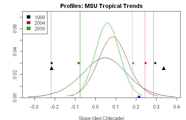


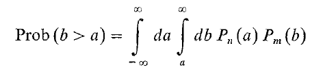
 , i.e. what bayesians call a “posterior distribution”, but I’m just learning the lingo. The dotted vertical lines represent 95% confidence intervals from the profile likelihood calculations shown in a prior post, color coded by endpoint. The colored dots represent 95% confidence intervals calculated using the Neff rule of thumb for AR1 autocorrelation in Santer. The black triangle at the bottom shows ensemble mean trend (0.214 deg C/decade).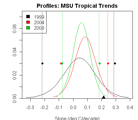

 . The dotted lines are as before; the solid color-coded vertical lines are the maximum likelihood trend estimates for the respective periods. Again for an analyst, the models seem to the the right of these estimates.