Zotero

Zotero is a Firefox add-on that, within the browser, can capture academic citations from Google Scholar, many library catalogues and multiple other sources. It permits you to insert links to the pdfs (both external and on your own directory) and go to them within the browser, to add your own cross-reference tags and notes. I began experimenting with it yesterday and have very quickly organized a lot of my references. It even appears to be WordPress compatible. It looks like this is a fantastic way of placing a bibliography online, which I anticipate doing at some point. I urge people who, like me, suffer from the chore of reference management to explore this tool

Ohio State

As Hu McCulloch mentioned, I am speaking tomorrow, Friday May 16, at OSU on “Was 1998 the Warmest Year of the Millennium: What do We Really Know?” The talk will be 2:30-3:48 in Scott Lab 001 (a big lecture hall in the basement of the south end of the east wing). A reception will follow. The talk is part of the Mechanical Engineering Seminar Series for graduate students, but there will be plenty of room for visitors.

Further details of the talk are at http://www.mecheng.osu.edu/me888/470/stephen-mcintyre-will-present-the-question-global-warming-what-do-we-really-know.

I just finished an interview on Fred Anderle’s WOSU-FM talk show “Open Line”, this morning 10:00-11:00 AM, along with Mohan Wali of OSU’s Dept. of Natural Resources and Environment. Hu says that an MP3 of the show will be online at http://www.wosu.org/radio/radio-open-line/ . FM 89.7, Columbus OH.

I’m looking forward to meeting Hu and others at OSU. As Hu surmises, I’ve been busy preparing for my talk, which is one reason why I’e been a bit quiet this week.

I don’t make many talks and always have a hundred more things that I want to say than I can.

Koutsoyiannis 2008 Presentation

Anything by Demetris Koutsoyiannis is always worth spending time on. Spence_UK draws our attention to this recent presentation at AGU asking:

How well do the models capture the scaling behaviour of the real climate, by assessing standard deviation at different scales. (Albeit at a regional, rather than global level).

Assessment of the reliability of climate predictions based on comparisons with historical time series (Click on “Presentation” to get through abstract page)

GISS Model E Data

Steve Mosher provides the following recipe for getting GISS Model E results:

Ok getting ModelE data

Start here http://data.giss.nasa.gov/

See the link for climate simulations of 1880-2003. click that

http://data.giss.nasa.gov/modelE/transient/climsim.html

Here you will see the link to the paper and all the readme I know of

now to get the data look at table 1.

See line #4. ALL FORCINGS. These are the similautions that include all forcings
( line 1-3 contain individual forcings, like GHG only for example, or volcano)

On the left hand side of the table you will see links for the forcing. On the RIGHT
you will see a list of RESPONSES.

select “lat time”

http://data.giss.nasa.gov/modelE/transient/Rc_jt.1.11.html

Now you will see a pull down menu.

See the first box. Quantity? Pick surface temp ( there are others as well )

Mean Peroid. pick 1 month to get rid of the running mean

Time interval: pick what you like.

base peroid. I selected 1961-1990 because I wanted to compare ModelE to hadcrut.

Output. Formatted page with download links

Show plot and then get the data

http://data.giss.nasa.gov/work/modelEt/time_series/work/tmp.4_E3Af8aeM20_1_1880_2003_1961_1990-L3AaeoM20D/LTglb.txt

Update: John Christy has sent in the following showing GISS Model E versus UAH. noting his regret that GISS had not reported their run a bit further out.

model_31.jpg

Where did IPCC 1990 Figure 7c Come From?

Here at Climate Audit, we occasionally try to solve mysteries that have vexed climate scientists for years. On a previous occasion, we helped UCAR locate the mysterious civilization of Chile, on another occasion the lost city of Wellington NZ and, most recently, helped NASA find the lost city of Cobija, Bolivia. Today we’ll help the climate science community identify the provenance of a graphic shown below, that was produced in 1990 by a mysterious organization known to insiders as IPCC.

lambh23.jpg
IPCC 1990 Figure 7c.

At his blog last year, William Connolley, obviously impressed with then recent CA success in locating Chile and Wellington NZ, appealed for help in solving this outstanding puzzle, specifically challenging me to identify its provenance for the climate science community, even accusing me of being “curiously uninterested in the source [of this graphic], or lack thereof” and worried that I was “ignoring” the provenance of this graphic, leaving the wider community to fend for itself.

One of his readers, obviously of the view that it was not necessarily my responsibility to sort out this particular IPCC conundrum, asked Connolley why he didn’t just determine who the IPCC author was and ask him:

Where does the 1990 graph come from then? I presume the IPCC author didn’t just hand draw it? Who is the IPCC lead author responsible, and if he is still alive, couldn’t one just ask?

This seems like a logical method, but Connolley was uninterested:

AFAIK it was hand drawn – it looks like it was. Its certainly not a computer plot. Things were free-and-easy back in ’90 I suppose (thought as far as I know this is the only graph from the ’90 report that does not have a good source) -W

At wikipedia, Connolley expounded further on the lack of a clear source for this graphic:

A schematic (non-quantitative) curve was used to represent temperature variations over the last 1000 years in chapter 7. The vertical temperature scale was labelled as “Temperature change (°C)” but no numerical labels were given; it could be taken to imply that temperature variations of the MWP and LIA were each of the order of 0.5 °C from the temperature around 1900. The section specifically states recent climate changes were in a range of probably less than 2 °C. The 1990 report noted that it was not clear whether all the fluctuations indicated were truly global (p 202). The graph had no clear source (it resembles figure A9(d) from the 1975 NAS report, which is sourced to Lamb, 1966), and disappeared from the 1992 supplementary report.

To say that I was “uninterested” in its source was untrue. This is the sort of thing that usually interests me, but I can’t solve every climate science puzzle instantaneously and on demand. On an earlier occasion, I posted up an extended excerpt from IPCC 1990, which is not available to many readers. However, I didn’t then know the source of the IPCC 1990 graphic, just as I don’t know how Mann calculated the MBH99 confidence intervals or many other small climate science mysteries.

Today I’m pleased to report that I think that I can report a solution to this small mystery, which I propose below. Continue reading

Southern Hemisphere Sea Ice Reaches "Unprecedented" Levels

Four of the past 5 months are “all-time” records for Southern Hemisphere sea ice anomalies, “unprecedented” since the data set began in 1979 as shown below:

On a global basis, world sea ice in April 2008 reached levels that were “unprecedented” for the month of April in over 25 years. Levels are the third highest (for April) since the commencement of records in 1979, exceeded only by levels in 1979 and 1982. This continues a pattern established earlier in 2008, as global sea ice in March 2008 was also the third highest March on record, while January 2008 sea ice was the second highest January on record. It was also the second highest single month in the past 20 years (second only to Sept 1996).

The graph below shows the monthly anomaly (aggregating NH and SH), collating information from ftp://sidads.colorado.edu/DATASETS/NOAA/G02135.
seaice98.gif
Figure 2. Monthly anomaly sea ice area.

As suggested by a reader, here’s the same information with each monthly series plotted as a separate line (April-solid; January – dotted.) The surge in anomaly area in 2008 is not limited to a single month, but is consistent for all 4 months to date (and for the YTD average).
seaice99.gif

At Cryosphere Today, they provide the following scientific description of recent sea ice changes:

You’ve heard Al Gore comment that the “Earth has a fever”? It may also have major tooth decay.

They provide an animation showing declining sea ice to 2007 lows, but not the subsequent recovery in 2008:

Peruse an archive of map displays of the atmospheric and radiative climatic conditions leading up to the record setting Northern Hemisphere sea ice minimum of 2007: sea ice autopsy

Instead of perhaps celebrating the dramatic recent increase in sea ice, they complain that there has been a loss of “multiyear sea ice”.

I’ve uploaded my collation of the NOAA data to http://www.climateaudit.org/data/ice/seaice.dat .

UODATE: NOAA reported high March 2008 SH sea ice here.

Raobcore Adjustments

One of the issues in play in criticisms of Douglass et al 2007 pertained to their use of RAOBCORE 1.2 rather than RAOBCORE 1.4.

As an editorial comment, since some critics of Climate Audit seem to feel that I bear some personal responsibility for defending this paper, I was not a co-author of Douglass et al nor I did not provide advice on it. I had not posted on it or reviewed it or even read it until a few days ago. Nor did I have any personal familiarity with radiosonde data sets. Nor had I followed the realclimate discussion of this article until a few days ago. I posted up a few days ago on tropical troposphere temperatures because of Ross McKitrick’s T3 concept and I merely did a simple plot of tropical troposphere temperature.

My proximate interest in this paper arose because this post prompted commentary on Douglass et al., including a statistical issue, previously raised by Gavin Schmidt (which I had not followed at the time), which was raised here by Beaker, which caught my interest. The idea of a climate scientist making a gross statistical error is something that would obviously not come as a total surprise to me, though I remain unconvinced that the particular issue advanced by Schmidt and endorsed by Beaker, concerning multi-model means, rises much above a play on words. In fact, my impression is it is more likely that Schmidt has committed the error, by confusing the real world with the output of a model, something that anthropologists have observed as something of an occupational hazard for climate modelers. (See discussion of Truth Machines here.)

The issues concerning radiosonde trends are more substantial, though Schmidt’s commentary is more oriented to proving a gotcha than a careful commentary on real issues pertaining to this data.

RAOBCORE is a re-analysis of radiosonde data by Leopold Haimberger and associates. RAOBCORE 1.2 was published in April 2007, though presumably available in preprint prior to that. Douglass et al 2007 was submitted in May 2007, when the ink was barely dry on the publication of RAOBCORE 1.2. Nonetheless, Schmidt excoriates Douglass et al for using RAOBCORE 1.2.

To date, RAOBCORE 1.4 has not been published in a peer-reviewed journal, though a discussion has been submitted (Haimberger et al 2008) and is currently online at Haimberger’s site. It was announced in Jan 2007 with Haimberger’s website stating that it used the “more conservative ERA-40 bg modification”. “Conservative”. I must say that I dislike the use of such adjectives by climate scientists. Dendros talk about “conservative” standardization, never about “liberal” standardization. Another adjective that sets my teeth on edge is “rigorous” as in a “rigorous statistical procedure”. Inevitably, such procedures are anything but.

RAOBCORE 1.4 data is online in a MSU gridded format at ftp://raobcore:empty@srvx6.img.univie.ac.at/v1_4/grid2.5_invd_1_6, with 24 different data sets covering combinations of 4 layers: tls=Lower Stratosphere (MSU4), tts=Troposphere-Stratosphere (MSU3), tmt=Mid-Troposphere (MSU2), tlt=Lower Troposphere; 3 versions: bg, tm and tmcorr; and two times: midnight (00) and noon (12). I’ve written a short program to extract this data and have made monthly time series for the tropics for all versions.

The underlying concept of the RAOBCORE re-analysis is to apply changepoint algorithms to detect inhomogeneities in the radiosonde record and there seems to be plenty of evidence that inhomogeneities are a real problem. So CA readers that are concerned about inhomogeneities in the surface record should not take the radiosonde record as written in stone, merely because they like the answer. Uncertainties in this record seem just as serious, if not more serious than uncertainties in the surface record.

I’ve done a quick assessment of the data, which has primarily involved figuring out how to download the data (which only goes to end 2006) and plotting the net adjustments in RAOBCORE 1.4 to the original data. (I haven’t located RAOBCORE 1.2 online yet.)

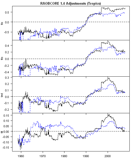
The difficulty that arises is that the recommended adjustments are typically of the same order of magnitude as the underlying trend and, in one case, larger than the underlying trend, such that the sign of the adjusted trend is different from the raw trend. First here is a figure showing the net adjustments for the tropics in deg C for the 4 levels (going high to low). In each case, the adjustments are implemented primarily in the 1985-2000 period, so one is not dealing with the far past. All records end in 2006 are not fully up-to-date.
raobco95.gif
Figure 1. RAOBCORE (tropics) adjustments for 4 levels 1957-2006. Black – midnight; blue- noon.

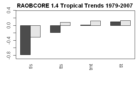
Next here is a figure showing the original and RAOBCORE 1.4 trends for the tropics for the 4 levels (version 1.2 is not shown). The sign in the MSU3 level is reversed by the adjustment process.
raobco94.gif

For completeness, here are plots showing the original and adjusted versions for the 4 levels.
raobco96.gif

It is evident from the above plots that the RAOBCORE adjustments are the same order of magnitude as the trend that people are seeking to determine.

Reference:
Haimberger L., 2007: Homogenization of Radiosonde Temperature Time Series Using Innovation Statistics. J. Climate, 20,1377- 1403 (April 2007) url

“No Working Papers”, “No Correspondence”

Last year, we noted the insolent and unresponsive answers by IPCC chapter 6 Lead Authors to Review Comments in connection with the Hockey Stick reconstructions. Under IPCC policies, Review Editors have important obligations to ensure responsiveness of Chapter Authors (see policies discussed here). The comments by Review Editors were not put online by IPCC, but, after some effort, David Holland managed to obtain the Review Comments for WG1 and WG2. While a few WG2 Review Editors made substantive comments, WG1 review editor comments proved to be a few-sentence form letter in all but one case (chapter 6 Review Editor Mitchell noting outstanding controversy in connection with the Hockey Stick.)

It seemed inconceivable that these form letters were the entire corpus of the Review Editor contributions, given their important obligations in the IPCC process. Holland accordingly pressed Mitchell for any supplementary information, reports pertaining to his duties as IPCC Review Editor. Even though IPCC policies state clearly that all comments will be retained for 5 years:

All written expert, and government review comments will be made available to reviewers on request during the review process and will be retained in an open archive in a location determined by the IPCC Secretariat on completion of the Report for a period of at least five years.

Mitchell replied that he had no kept “any” working papers and that he was not required to do so.

For my own part, I have not kept any working papers. There is no requirement to do so, given the extensive documentation already available from IPCC.

In the modern day and age, it seemed inconceivable that Mitchell could have discharged his duties without any trace or ripple in the electronic pond and accordingly, on April 1, 2008, Holland submitted an FOI request asking for all emails to and from Dr Mitchell in his capacity as IPCC Review Editor, with a turn of phrase that unfortunately was construed as limiting the request to emails concerning the HS. Once again, he has been essentially stonewalled. Although Mitchell’s final terse Review Editor report referred to outstanding issues in connection with the HS, according to the Met Office, Mitchell either never corresponded with any IPCC chapter author or IPCC official about these misgivings during the course of the IPCC review process or subsequently destroyed the relevant correspondence. Continue reading

David Douglass' Comments:

David Douglass writes in: Continue reading

Ice Ages #2