-
Tip Jar
-
Pages
-
Categories
-
Articles
-
Blogroll
- Accuweather Blogs
- Andrew Revkin
- Anthony Watts
- Bishop Hill
- Bob Tisdale
- Dan Hughes
- David Stockwell
- Icecap
- Idsos
- James Annan
- Jeff Id
- Josh Halpern
- Judith Curry
- Keith Kloor
- Klimazweibel
- Lubos Motl
- Lucia's Blackboard
- Matt Briggs
- NASA GISS
- Nature Blogs
- RealClimate
- Roger Pielke Jr
- Roger Pielke Sr
- Roman M
- Science of Doom
- Tamino
- Warwick Hughes
- Watts Up With That
- William Connolley
- WordPress.com
- World Climate Report
-
Favorite posts
-
Links
-
Weblogs and resources
-
Archives
Tropical Troposphere
Apr 26, 2008 – 12:16 PM
Last year, Ross McKitrick proposed the ironic idea of a “T3 Tax” in which carbon tax levels were related to observed temperature increases in the tropical troposphere. Temperature increases in the tropical troposphere are, as I understand it, a distinctive “fingerprint” for carbon dioxide forcing. Apparent discrepancies between a lack of warming in satellite data and surface warming have been a battleground issue for many years. In one of the most recent surveys of the matter in 2006, the U.S. CCSP proclaimed that the issue had been put to rest:
Previously reported discrepancies between the amount of warming near the surface and higher in the atmosphere have been used to challenge the reliability of climate models and the reality of human induced global warming. Specifically, surface data showed substantial global-average warming, while early versions of satellite and radiosonde data showed little or no warming above the surface. This significant discrepancy no longer exists because errors in the satellite and radiosonde data have been identified and corrected. New data sets have also been developed that do not show such discrepancies.
In this respect, the March 2008 satellite data for the tropics is pretty interesting. The graph below shows UAH (black) and RSS (red) for the tropics (both divided by 1.2 to synchronize to the surface variations – an adjustment factor that John Christy said to use in an email). I also collated the most recent CRU gridded data and calculated a tropical average for 20S to 20N, shown in green. All series have been centered on a common interval.

Figure 1. Tropic (20S-20N) temperatures in [anomaly] deg C. All data shown to March 2008. Script for calculations is given in #19 below. Reference periods for original data converted to reference period 1979-1997 here.
There have only been a few months in the past 30 years which have been as cold in the tropical troposphere as March 2008 four months in the 1988-1989 La Nina. At present, there is no statistically significant trend for the MSU version. The data set has very high autocorrelation (but I note that autocorrelation doesn’t represent the spikes very well.)
Obviously each fluctuation is unique – I presume that we’ll see some sort of behavior in the next 18 months like after the 1988-1989 Nina – so that one can reasonably project that the long-term “trend” as at the end of 2009 will be a titch lower than the trend as calculated today.
While RSS and UAH move together, there is a slight drift upwards in RSS relative to UAH and there’s still a slight trend in the RSS numbers. There’s a third data set (Vinnikov – Maryland) which is not kept up to date, which has trends higher than either. Even CRU is now reporting tropical temperatures at surface that are below average during this period.
I draw no conclusions from this other than some claims about the statistical significance of trends need to be examined. The autocorrelation of the data set is very high; although I’m not in a position to pronounce on the matter, the concerns expressed by Cohn and Lins about long-term persistence seem highly pertinent to the sort of patterns that one sees here. Some readers may note a graphic in summer 2005 .
realclimate discusses the issue up to Dec 2007 here. Since then, cooling has been 0.3-0.4 deg C in UAH and MSU.
UPDATE: This post has occasioned references to Douglass et al 2007. Here is Table IIa from that paper.

Anthony Watts at NCDC
Apr 26, 2008 – 7:51 AM
Anthony has two interesting reports on his NCDC visit. Take a look.
MBH99 and Proxy Calibration
Apr 23, 2008 – 12:03 PM
UC and Hu McCulloch have been carrying on a very illuminating discussion of statistical issues relating to calibration , with UC, in particular, drawing attention to the approach of Brown (1982) towards establishing confidence intervals in calibration problems.
In order to apply statistical theory of regression , you have to regress the effect Y against the cause X. You can’t just regress a cause X against a bunch of effects Y, which is what Wilson did in Kyrgyzstan and occurs all too frequent in paleoclimate, without a proper consideration of the effect of the inverse procedure.
Calibration deals with the statistical situation where Y is a “proxy” for X and where you want to estimate X, given Y. It’s the kind of statistics that dendros should be immersing themselves in, but which they’ve totally disregarded, using instead procedures for estimating confidence intervals that cannot be supported under any statistical theory – a practice unfortunately acquiesced in by IPCC AR4, hardly enhancing their credibility on these matters.
The starting point in Brown (1982) is the following:
Perhaps the simplest approach is that of joint sampling. It is easy to see that given α, β, σ, X, X’, the joint sampling distribution of is such that:
is standard normal. Note that this standard normal does not involve any of the conditioning parameters α, β, σ, X, X’ so that probability statements are also true unconditionally and, in particular, over repetitions of (Y,X) where both Y and X are allowed to vary.
I dare say that many readers may find that this statement is a fairly big first bite and that it may not be as obvious to them as to Brown’s audience.
However, this particular result is derived in chapter 1 of a standard textbook, Draper and Smith, Applied Regression Analysis (1981). I worked through this chapter in detail and found the exercise very helpful. Its’ approach is, in turn, derived from E.J. Williams (1959), Regression Analysis, chapter 6. In some fields, while people “move on”, they try to at least achieve results that survive the test of time.
The key strategy in the univariate cases is to draw curves enclosing the 100(1-γ) confidence intervals for y given x. These are quadratic in x. Illustrations are given in Draper and Smith Figures 1.11 and 1.12 and Williams Figure 6.2. The equation for the confidence interval curves is:
where t is the 100(1-γ) t-statistic for the relevant degrees of freedom, for the calibration set and the others are usual estimators.
This can be transformed to a quadratic equation in x. The strategy in these texts for estimating fiducial limits on x given y is to draw a horizontal line at y, determine the intersections with the two confidence interval curves and take the x-values of the intersection as the upper and lower fiducial limits, with the estimate being calculated from the fitted linear equation:
In a “well behaved case”, the upper confidence limit is on the upper quadratic and the lower confidence limit is on the lower quadratic and the estimate is between the upper and lower confidence intervals. However, if the roots to the quadratic are complex, there are no solutions to the equation, which means that any value of x falls within the confidence limits permitted from the data. Another related pathological case arises when both the “upper” and “lower” confidence intervals are on the same side of the estimate.
In these cases, if one examines the regression fit in univariate calibration, one finds that there was no statistically significant fit and in effect could not be statistically differentiated from zero. This is a point that UC has been emphasizing in recent posts.
I went through all 14 MBH99 proxies and found that they beautifully illustrated the pathologies warned about in these texts.
First here is an example where the calibration graphic in the style of Draper and Smith 1981 has the structure of a “well behaved” calibration. This is for Briffa’s Tornetrask series. The calibration here has been “enhanced” by some questionable prior manipulations by Briffa, who constructed his temperature series by an inverse regression of regional temperature against 4 time series – so the “raw” proxy is not really “raw” any more. In these graphics, I’ve used the average value of the proxy in the 1854-1901 “verification” period as the y-value (everything’s been standardized on 1902-1980). In this case, the fiducial limits for x (temperature) given y are 0.36 deg C, so this looks like a pretty successful calibration (BUT the prior massaging will have to be deconstructed at some point.)
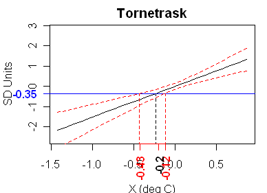
Figure 1. Proxy value (as in other figures) is in SD Units; X-axis in deg C.
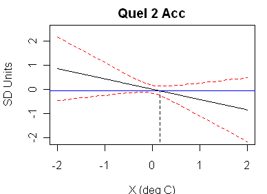
Next here is the same style of diagram for the Quelccaya 2 accumulation series, showing a very pretty example of complex roots and no fiducial limits. Examining the original calibration regression, one finds an r^2 of 0.011 (Adjust r^2 of -0.00147) with an insignificant t-statistic of -0.94 for the proxy-temperature relationship. Because the coefficient is not distinguishable from 0, there is no contribution towards calibration from this data.
Here’s a snippet of the corresponding Draper -Smith from Google, which shows enough that you can see that the Quelccaya 2 Accumulation case matches the situation in the Draper Smith Figure 1.12 top panel diagram.
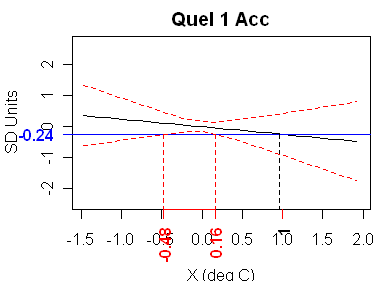
Quelccaya 1 accumulation is also pathological but, in this case, the quadratic solves, but the both the “upper” and “lower” confidence intervals are on the same side of the estimate, as shown below. This calibration also fails standard tests, as the t-statistic is -0.544 (the r^2 is less than 0.01).
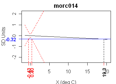
Here’s another pretty example of total calibration failure – the morc014 tree ring series. This would make a nice illustration in a statistics text. This has a t-statistic of -0.037 – a value that is low even for random series.
In total, 10 of the 14 series in the MBH99 failed this chapter 1 calibration test. In addition to the above 3 series, other failed series were: the fran010 tree ring series, Quelccaya 1 dO18, Quelccaya 2 dO18 (why are there 4 different Quelccaya series??), a Patagonia tree ring series, the Polar Urals reconstruction and the West Greenland dO18 series.
Only 4 series passed this elementary test. In addition to the highly massaged Tornestrask series, the three were: the Tasmania tree ring series, the NOAMER PC2 and the NOAMER PC1 (AD1000 style.) I guess the Tasmania series teleconnects to NH temperature more than most of the NH tree ring reconstructions. Its calibration results are not strong – the t-statistic is 2.1 and the adjusted r^2 is 0.04.
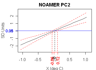
Now to what we’ve been waiting for: the NOAMER PC series. The NOAMER PC2 (and the AD1000 network is far more dominated by Graybill bristlecones than even the AD1400 network) has the strongest fit. It has a t-statistic of 4.3 and an adjusted r^2 of 0.19, the highest in the network.
And what does this high-correlation reconstruction look like? Not very HS, that’s for sure.
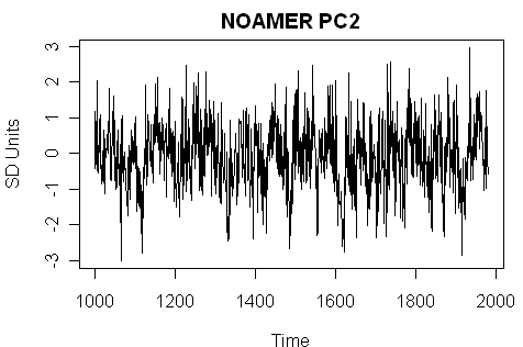
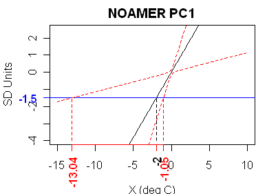
Now what of the NOAMER (Graybill bristlecone) PC1? This is the only MBH99 series that has a HS shape (I’ve flipped the archived series so that it has the expected upward bend). It has a very idiosyncratic appearance in the Draper-Smith style diagram as shown below. The upper and lower limits are on opposite sides of the estimate, but this series yields very broad fiducial limits. The t-statistic here is 1.71, somewhat below statistical significance. The MBH99 “adjustment” of the PC1 has the effect of “improving” its fit to temperature, and thereby increasing its weight in an MBH-style reconstruction.
Moving towards Multivariate Calibration
As we approach the mountain of multivariate calibration, let’s pause and consider the information on fiducial limits from the 4 series that actually calibrated, as summarized in the table below:
| Proxy | Lower (deg C) | Upper (deg C) |
| NOAMER PC1 | -13.04 | -1.05 |
| Tornetrask | -0.43 | -0.12 |
| NOAMER PC2 | -0.06 | 0.12 |
| Tasmania | 0.09 | 1.04 |
Thus, we have the remarkable situation where the 95% fiducial limits for the 4 proxies essentially do not overlap at all (there’s a miniscule overlap between the NOAMER PC2 and Tasmania). It will be interesting to see what happens as one works through a Brown 1982 style calibration. It also illustrates rather nicely the total lack of significance of the majority of proxies.
It’s hard to think how one can purport to derive confidence intervals of a few tenths of a degree, when 10 of 14 proxies don’t calibrate at all and the remaining 4 yield results that are inconsistent in the verification period.
I did these calculations with the MBH “sparse” temperature series since it had a verification value. MBH obviously used temperature PCs for calibration. Even though the two series are highly correlated, the calibrations will be different though I’d expect the patterns to stay pretty similar.
Wilson in Kyrgyzstan
Apr 23, 2008 – 6:54 AM
Wilson et al 2007 (previously discussed here) considers a Kyrgyzstan series that has numerous issues – the usual provenance problems unfortunately occur once again. But over and above that, it uses multiple inverse regression, a procedure used all too casually by dendros. In this case, the procedure flips over one of the ring width series and results in the reconstruction having a substantially higher 20th century trend than any of the constituent series. The form of multiple inverse regression is a little different than Mannian inverse regression and arguably even worse. Also when I replicated the recon using ITRDB chronologies, I got quite different (higher) results in the 18th century and no 20th century trend. Continue reading
Rob Wilson and the Yamal Divergence
Apr 21, 2008 – 9:19 AM
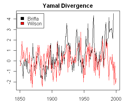
The archived information for Wilson et al 2007 contains interesting new information on an unpublished West Siberian series (Putorama, 70 31 N, 92 57E). In this case, I was actually able to obtain a better correlation to gridcell temperature than the one reported by Rob by using a gridcell closer to the actual location. This series has no 20th century trend. Wilson noted a divergence from instrumental records at the end of the record. However, there is a remarkable divergence between the new West Siberian series which is touching lows at its end and the West Siberian series beloved by multiproxy reconstructions (Briffa’s Yamal series), which touches new highs at the end of its record.
Rob reported the following:
This series correlates with mean May–September gridded temperatures at 0.43 (Table 1). The Western Siberia series tracks the gridded temperature series quite well (Figure 3) except for the last two years, where the proxy values are substantially lower than the actual instrumental data. These two years of misfitting are too short to identify whether this is a significant divergence.
The temperature comparison was said to be to two gridcells (62-67N; 82E) over the period 1938-2000. However, there are available gridded values from 1881 on for the gridcell 67N, 87E (derived mainly from Turuhansk 66N 89E), obviously much closer to Putorama than the gricells used in the study. The correlation to the Turuhansk gridcell (over 1881-2000 exccept for a few years) for the May-Sept period specified in Table 1 was 0.54 – better than the reported values.
Here is a plot comparing the tree ring and gridded temperature series. While there is a good correlation to temperature, there is also no 1920-2000 trend in the tree ring data (actually slightly negative.)
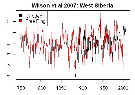
Figure 1, Both series scaled to SD units.
Rob noted that the data tracked well “except for the last two years” where there is a divergence. Visually, it looked to me like the divergence was more than just the last two years. Below is a plot of the residuals from a fit of RW against gridded temperature. While the negative residuals are more pronounced in the past few years, there does appear to be somewhat of a negative divergence trend in the residuals for more than the past two years. The Durbin-Watson statistic using the lmtest package in R was 1.50 – right at the red zone value – and differs substantially from the reported DW value of 1.98. I wonder how Rob calculated his DW statistic.
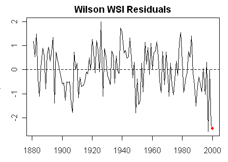
Figure 2. Residuals from fit to gridded temperature – in SD units.
Now for the most interesting divergence. I’ve discussed the Yamal series (Briffa variation) on many occasions. This is a staple of multiproxy studies and is individually shown in the IPCC AR4 spaghetti graph. Although the Yamal chronology is usually attributed to Hantemirov (2002) e.g. by Juckes et al 2007, the staple version was calculated by Briffa, who has only reported the chronology and refused to provide the supporting measurement data. It has a pronounced HS shape with its medieval-modern differential very different from the Polar Urals Update. While the Putorama series is some distance to the east of the Yamal-Urals series, any new light on West Siberian chronologies is welcome.
The figure below compares the Briffa Yamal version with the new Wilson et al chronology. Whereas the Briffa chronology is exploring new highs at its close, the Wilson West Siberian series is exploring new lows. One looks forward to the commentary if and when a study is published on the new West Siberian chronology.
"Correlates well (r = 0.70) with gridded June–July temperatures"
Apr 20, 2008 – 8:50 PM
I’ve been re-visiting some proxy data; I noted last summer that Rob Wilson had archived a considerable amount of B.C. data in Aug 2007 and noticed that he subsequently archived the data versions as used in Wilson et al 2007 at NCDC here in Sept 2007. (Not all of Rob’s data is archived as he isn’t in control of all the data that he’s been involved with; for example, Brian Luckman of the University of Western Ontario is holding out on archiving data, notwithstanding commitments of the IAI program discussed here.
Wilson et al 2007 attempts to argue that the Divergence Problem is not necessarily as bad as it seems. They calculate a composite over the period 1750-2000 (so it’s relatively up-to-date) and, perhaps responding somewhat to criticisms from CA about the overuse of stereotypes, set as one of their criteria that the proxy not have been included in prior compilations.
There are many aspects of the methodological description that are better than has been traditional in the field, though the descriptions are far from perfect. Unfortunately, despite many promising features, efforts to replicate results using published descriptions and data quickly foundered. Continue reading
The RE Benchmark of 0
Apr 17, 2008 – 1:02 PM
In MM2005a,b,c, we observed that the RE statistic had no theoretical distribution. We noted that MBH had purported to establish a benchmark by simulations using AR1 red noise series with AR1=0.2, yielding a RE benchmark of 0. We originally observed that high RE statistics could be obtained from PC operations on red noise in MM2005a (GRL) simply by doing a regression fit of simulated PC1s on NH temperature. Huybers 2005 criticized these simulations as incompletely emulating MBH procedures, as this simulation did not emulate a re-scaling step used in MBH (but not mentioned in the original article or SI). In our Reply to Huybers, we amended our simulations to include this re-scaling step, but noted that MBH also included the formation of a network of 22 proxies in the AD1400 step and if white noise was inserted as the other 21 proxies, then we once again obtained high (0.54) 99% benchmarks for RE significance. Our Reply fully responded to the Huybers criticism.
Wahl and Ammann/Ammann and Wahl consider this exchange and, as so often in their opus, misrepresent the research record.
Before I discuss these particular misrepresentations, I’d like to observe that, if I were re-doing the exposition of RE benchmarking today, I would discuss RE statistics in the context of classic spurious regression literature, rather than getting involved with tree ring simulations. This is not to say that the simulations are incorrect – but I don’t think that they illuminate the point nearly as well as the classic spurious regressions (which I used in my Georgia Tech presentation.)
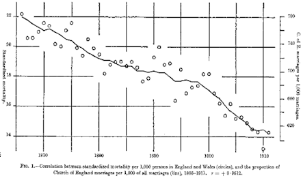
The classic spurious regression is in Yule 1926, where he reported a very high correlation between mortality and the proportion of Church of England marriages, shown in the figure below. Another classic spurious regression is Hendry 1980’s model of inflation, in which he used cumulative rainfall to model the UK consumer price index. In both cases, if the data sets are divided into “calibration” and “Verification” subsets, one gets an extremely “significant” RE statistic – well above 0.5. Does this “prove” that there is a valid model connecting these seemingly unrelated data sets? Of course not. It simply means that one cannot blindly rely on a single statistic as “proof” of a statistical relationship.
In effect, the RE statistic has negligible power to reject a classic spurious regression.
This seems like a pretty elementary point and I don’t know why it’s so hard for so many climate scientists to grasp in the case of the proxy literature.
Wahl and Ammann/Ammann and Wahl wade blindly into this. They don’t spend any time examining primary literature on bristlecones to prove that Graybill’s chronologies are somehow valid. They don’t discuss the important contrary results from the Ababneh 2006 thesis, although you’d think that they or one of the reviewers would have known of these results.
Instead, they try to resuscitate an RE benchmark of 0, by making several important misrepresentations of both our results and MBH results.
Wahl and Ammann 2007 states (Appendix 1):
When theoretical distributions are not available for this purpose, Monte Carlo experiments with randomly-created data containing no climatic information have been used to generate approximations of the true threshold values (Fritts, 1976; cf. Ammann and Wahl, 2007; Huybers, 2005; MM05a, MM05c—note that the first two references correct problems in implementation and results in MM05a and MM05c).
MM05c is our Reply to Huybers. Obviously Huybers 2005 could not “correct problems in implementation and results in MM05a and MM05c” since MM05c was a reply to Huybers 2005. In fact, in my opinion, MM05c completely superceded Huybers 2005 as it obtained high RE values with re-scaling in the context of an MBH network – a more complete emulation of MBH methods than Huybers 2005. Ammann and Wahl seem almost constitutionally incapable of making accurate statements in respect to our work.
Ammann and Wahl 2007 is later than MM05c. Did it or Wahl and Ammann 2007 “correct” any “errors in implementation” in MM05c?
Wahl and Ammann 2007 Appendix 2 makes the following criticism of our method of simulating synthetic tree ring series:
one byproduct of the approach is that these time series have nearly uniform variances, unlike those of the original proxies, and the PCs derived from them generally have AC structures unlike those of the original proxies’ PCs. Generally, the simulated PCs (we examined PCs 1–5) have significant spurious power on the order of 100 years and approximate harmonics of this period. When the original relative variances are restored to the pseudoproxies before PC extraction, the AC structures of the resultant PCs are much like those of the original proxy PCs.
Here I don’t exactly understand what they did and, as I presently understand this sentence, it doesn’t make much sense in an MBH context. In Mannian PCs (or correlation PCs), the time series are standardized to have uniform standard deviations (and thus variance) in the calibration period (and entire period respectively). So even if the variance of the time series in our network were too uniform (and I haven’t analyzed whether this is so or not as yet, I don’t see how this could affect the downstream calculations for Mannian pseudo-PCs or correlation PCs. I don’t get the relevance of this point even if it were valid.
Later in the paragraph in Apendix 2, they seem to concede this:
Using the AC-correct PC1s in the RE benchmarking algorithm had little effect on the original MM benchmark results, but does significantly improve the realism of the method’s representation of the real-world proxy-PC AC structure.
So if this observation – whatever it is – had “little effect” on the original results, so what?
Even though Ammann and Wahl 2007 acknowledged that MM2005c (Reply to Huybers) contained the most detailed exposition of RE simulation results:
Particularly, MM05c (cf. Huybers 2005) have evaluated the extent to which random red-noise pseudoproxy series can generate spurious verification significance when propagated through the MBH reconstruction algorithm.
Wahl and Ammann 2007 totally failed to consider the methods described in MM05c, instead merely repeating the analysis of Huybers 2005 using a network of one PC1 rather than a network of 22 proxies (a PC1 plus 21 white noise series as in MM05c). They purported to once again get a RE benchmark of 0.0:
When we applied the Huybers’ variance rescaled RE calculation to our AC-correct pseudoproxy PCI s, we generated a 98.5% significance RE benchmark of 0.0.
But note the sleight of hand. MM2005c is mentioned, but they fail to show any defect in the results. They misrepresent the research record by claiming that Huybers 2005 had refuted MM2005c – which was impossible – and then they themselves simply replicate Huybers’ results on a regression network of one series and not a full network of 22 series. Also it’s not as though these matters weren’t raised previously. They were. It’s just that Ammann and Wahl didn’t care.
They also make an important misrepresentation of MBH. Ammann and Wahl 2007 (s4) asserts:
MBH and WA argue for use of the of Reduction of Error (RE) metric as the most appropriate validation measure of the reconstructed Northern Hemisphere temperature within the MBH framework, because of its balance of evaluating both interannual and long-term mean reconstruction performance and its ability thereby to avoid false negative (Type II) errors based on interannual-focused measures (WA; see also below).
In respect to MBH, this claim, as so often in Ammann’s articles about Mann, is completely untrue. MBH did not argue for the use of the RE statistic as the “most appropriate” validation measure “because of its balance of evaluating both interannual and long-term mean construction…”. These issues did not darken the door of MBH. As reported on many occasions, MBH Figure 3 illustrated the verification r2 statistic in the AD1820 step, where they say that it passed. If MBH had reported the failed verification r2 in other steps and attempted to argue a case for preferring the RE statistic as Wahl and Ammann are now doing, then one would have more sympathy for them. But that’s not what they did. They failed to report the failed verification r2 statistic. And now Ammann is simply adding more disinformation to the mix by falsely asserting that MBH had argued for a justification that was nowhere presented in the four corners of MBH.
By discussing these particular misrepresentations, please don’t take that as a complete inventory. It’s hard to pick all the spitballs off the wall and these are merely a couple of them. I’ll discuss more on other occasions.
As I noted elsewhere, I’ve written to Ammann asking him for a statistical reference supporting the statement:
Standard practice in climatology uses the red-noise persistence of the target series (here hemispheric temperature) in the calibration period to establish a null-model threshold for reconstruction skill in the independent verification period, which is the methodology used by MBH in a Monte Carlo framework to establish a verification RE threshold of zero at the > 99% significance level.
So far no support has been provided for this claim.
8500-Year Old Tree Found in Sweden
Apr 17, 2008 – 8:56 AM
A news report says that the oldest living tree has been found on the Sweden-Norway border.

The report comes from Leif Kullman, a prominent Swedish paleo-scientist. The story says:
Prof Leif Kullman at Umeå University and colleagues found a cluster of around 20 spruces that are over 8,000 years old. The oldest tree, in Fulu Mountain, Dalarna (“the dales”), was dated by carbon dating at a laboratory in Miami, Florida to 9,550 years old and around it were generations of clones 375, 5,660 and 9,000 years old that have the same genetic makeup. The clones take root each winter as snow pushes low lying branches of the mother tree down to ground level, explains Prof Kullman.
“A new erect stem emerges, and it may lose contact with the mother tree over time.”
The trunks of the mother tree would survive only around 600 years but the trees are able to grow a new one, he adds. The finding is surprising because the spruce tree has been regarded as a relative newcomer in the Swedish mountain region and is thought to have originated 600 miles away in the east.
“Our results have shown the complete opposite, that the spruce is one of the oldest known trees in the mountain range,” says Prof Kullman.
Ten millennia ago, a spruce would have been extremely rare and it is conceivable that the ancient humans who lived there imported the tree, he says.
“Man immigrated close to the receding ice front. We have also found fossil acorns in this area, and people may have taken them with them as they moved over the landscape.”
It had been thought that this region was still in the grip of the ice age but the tree shows it was much warmer, even than today, he says.
“Spruces are the species that can best give us insight about climate change,” he says.
The summers 9,500 years ago were warmer than today, though there has been a rapid recent rise as a result of climate change that means modern climate is rapidly catching up.
The tree probably survived as a result of several factors: the generally cold and dry climate, few forest fires and relatively few humans. Today, however, the nature conservancy authorities are considering putting a fence around the record breaking tree to protect it from trophy hunters.
I can’t tell from this description whether the mother tree will yield a complete chronology; visually it looks smaller than the old bristlecones. If they’re talking about a continuous clone, then I think that there are other examples of such a phenomenon of similar age – I recall seeing something about cactus.
Tornetrask, which we’ve discussed on a number of occasions, is also located in Sweden. Grudd has a new Tornetrask reconstruction, which I’ve requested a digital version of – so far unsuccessfully and without a response.
In a post a couple of years ago, I mentioned what happened to the previous holder of the record as oldest living tree:
To facilitate compilation of a long-term tree-ring chronology for the Wheeler Peak area, one of the larger living bristlecone pines was sectioned. This tree, WPN-114, grew at an altitude of 10,750 feet on the gently sloping crest of a massive lateral moraine of Pleistocene age. The site was relaitvely stable during the lifetime of the tree, the only appreciable change being an accumulation of avalanche-transported debris so that the present ground surface is about 2 ft above the original base of the tree.
