Hansen Step 2 – First Thoughts

The source code for Hansen’s Step 2- the “urban adjustment” step is online. If anyone’s been able to operate the program through to Step 2, I’d be interested in some stage results for the stations discussed here. The verbal description is not clear and the code is a blizzard of old-fashioned Fortran subscripts, so it will take a little while to translate the procedure into modern languages and see what he’s doing.

Hansen et al 1999 says:

An adjusted urban record is defined only if there are at least three rural neighbors for at least two thirds of the period being adjusted. All rural stations within 1000 km are used to calculate the adjustment, with a weight that decreases linearly to zero at distance 1000 km.

In the stations that I’ve looked at, I’ve seen adjusted stations being calculated when the above condition doesn’t seem to hold. So any light that can be shed on the procedures would be appreciated.

Stations within 1000 km
The first step in Hansen’s Step 2 is the calculation of rural stations within 1000 km of an urban station to be adjusted. The archived script shows that this calculation is done from scratch in each run. No particular harm in that although the information presumably remains the same in every run. I’ve compiled the list of “Hansen-rural” stations for each of the 7364 stations, including in each list the id, name, lat, long, start_raw, end_raw, start_adj, end_adj, distance (from target), GISS-population, GISS-urban and GISS-lights. I archived the result at http://data.climateaudit.org/data/giss/stat_dist.tab . The information is a bit redundant to the station information lists but it was handy having some of the information directly accessible to aid analysis. The object is 33MB . The script to do this is at http://data.climateaudit.org/scripts/station/hansen/step2A.txt

In order to analyze Hansen’s actual urban adjustment mechanism, it’s nice to identify the stations with only a few contributing rural stations. There’s a very pretty R function that can do this in one line. The object containing the information stat_dist.tab is structured as a list in R with 7364 items, one for each GISS station. Each item is an R data-frame – which is structured as a matrix but the columns can be of different types. A very handy thing to be able to use. To obtain the number of rows for the 1000th station in the list, you can use the command

nrow(stat_dist[[1000]]) #86

To obtain the number of rows for all 7364 stations, all you need to do to get a vector is:

stat.length=sapply(stat_dist,nrow)

Just like magic. No blizzard of Fortran subscripts and 5 pages and programming.

Now to locate stations with only a few contributing rural stations for analysis purposes, you can do the following (I’ve already got my GISS information http://data.climateaudit.org/data/station/giss/giss.info.dat loaded as stations.tab

temp=(stat.length<3) ; index=(1:7364)[temp]
temp_urban=(stations$urban==”U”)
stations[temp&temp_urban,1:10]

This yields the following list of sites, all in India:

country id name lat long altitude alt.interp urban pop topo
1180 207 20742867000 NAGPUR SONEGA 21.1 79.05 310 302 U 930 HI
1188 207 20743128000 BEGAMPET 17.5 78.50 545 550 U 1796 HI
1190 207 20743185000 MACHILIPATNAM 16.2 81.15 3 30 U 113 FL

In these three cases, I checked and there was no “adjusted” series for any of the 3 sites, which, in this case, complies with the Hansen et al 1999 3-rural station criterion. I then checked “U” sites with 3 neighbors, all in India, Brazil and New Zealand and again didn’t obtain any adjusted series.

index=(1:7364)[temp_urban& (stat.length==3)];stations[index,1:10]

country id name lat long altitude alt.interp urban pop
1189 207 20743149000 CWC VISHAKHAP 17.70 83.30 66 142 U 353
2054 303 30382599000 NATAL AEROPOR -5.92 -35.25 52 12 U 377
2062 303 30382900000 RECIFE -8.05 -34.92 7 18 U 1184
2088 303 30383781000 SAO PAULO -23.50 -46.62 792 883 U 7034
6011 507 50793116001 AUCKLAND -36.90 174.80 5 9 U 145
6012 507 50793116002 ALBERT PARK -36.85 174.77 49 4 U 145
6013 507 50793116003 AUCKLAND, ALBERT PARK -36.85 174.77 49 4 U 145
6014 507 50793119000 AUCKLAND AIRP -37.02 174.80 6 17 U 145
6024 507 50793890001 DUNEDIN AERODROME -45.93 170.20 1 151 U 77
6025 507 50793893001 DUNEDIN MUSSELBURGH NEW ZE -45.90 170.50 2 190 U 77

I then experimented with sites classified as “small” and got some puzzles as shown below.

index=(1:7364)[temp_small& (stat.length==3)];stations[index,1:10]

country id name lat long altitude alt.interp urban pop topo
312 125 12567197000 FORT-DAUPHIN -25.03 46.95 9 100 S 14 HI
1185 207 20743041000 JAGDALPUR 19.08 82.03 553 512 S 47 HI
1855 224 22443436000 BATTICALOA 7.72 81.70 12 8 S 42 FL
1861 224 22443497000 HAMBANTOTA 6.12 81.13 20 42 S 11 FL
6023 507 50793844000 INVERCARGILL -46.70 168.55 4 28 S 49 FL

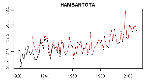
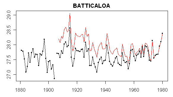
For the first two sites, there was no adjusted series, but for the 3-5 series there were adjusted series. Batticaloa and Hambantota are very close and it turns out that their 3 R neighbors are identical. So based on the apparent Hansen adjustment process in which the urban station trends are supposedly coerced to the rural reference stations, one would expect similar adjusted trends. This proves not to be the case. Why – I’m not sure right now and would welcome any thoughts.

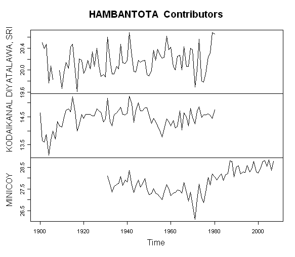
The three rural stations for Batticaloa and Hambantota are shown below – note that the distances from the two urban sites to the three rural comparanda are similar and in the same order.

id name long lat start_raw end_raw start_adj end_adj dist pop urban lights
1859 22443476001 DIYATALAWA, SRI 81.00 6.80 1901 1980.917 1901 1980.917 128.2031 NA R A
1200 20743339000 KODAIKANAL 77.47 10.23 1900 1980.917 1900 1980.917 542.0993 NA R A
1203 20743369000 MINICOY 73.15 8.30 1931 2007.917 1931 2007.917 943.8923 NA R A

id name long lat start_raw end_raw start_adj end_adj dist pop urban lights
1859 22443476001 DIYATALAWA, SRI 81.00 6.80 1901 1980.917 1901 1980.917 76.9864 NA R A
1200 20743339000 KODAIKANAL 77.47 10.23 1900 1980.917 1900 1980.917 609.3207 NA R A
1203 20743369000 MINICOY 73.15 8.30 1931 2007.917 1931 2007.917 913.2765 NA R A

The figure below shows the annual temperature values of the three rural stations. Two of them end in 1980 and only one (Minicoy) continues to the present). I test the proportion of years with at least 3 stations to the number of years of adjusted record and found that 2 of the 3 series failed the test. So it would be interesting to locate exactly where Hansen implements the 2/3 criterion in his code. I haven’t been able to do so yet. One also sees that, in this case, much depends on the Minicoy station as the only one continuing to the present.

wellin59.gif

Now for today’s puzzle – showing the dset=1 and adjusted versions of Hambantota and Batticola. How does Hansen get such different looking adjustments from identical rural comparanda? If anyone can do runs of the actual code for these stations and save any intermediate work, it would help. (Also Wellington NZ).

wellin58.gif

wellin60.gif

Help NASA Find the Lost City of Wellington NZ

Last spring, we offered to help UCAR locate the mysterious lost civilization of Chile. I reported:

If one goes to the ds570.0 location, http://dss.ucar.edu/datasets/ds570.0/data/ (you may have to register), there is a map of the world which appears to be comprehensive (i.e. all known oceans and continents are displayed.) Above the map is the following intriguing message:

Click region for station list. There are also non-WMO stations and stations with no location .
..
A number of the mystery stations came from the mysterious civilization known as “Chile”, whose existence has long been suspected. … Other lost civilizations include the mystery lands of Barbados and Argentina. I guess that it will be up to archaeologists to locate the intriguingly named “Bogus Station”. Is it in the depths of the Taklamakan desert, in an unknown oasis surrounded by a few hardy Dulan junipers known only to dendroclimatologists seeking temperature proxies? As noted above, CA readers are generous with their time and ideas. If you can solve these thorny problems, I’m sure UCAR will be very grateful.

CA readers suggested to UCAR that there were clues that the mysterious lost civilization of Chile was located in South America, but when I checked, UCAR still regarded Chile as being a lost civilization.

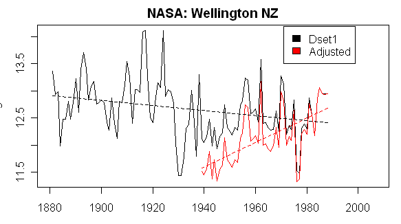
Today I invite CA readers to solve another mystery: help NASA locate the lost city of Wellington NZ. Here is a plot showing NASA dset=1 and adjusted data for Wellington NZ. As you see the data has not been updated since 1988! So let’s help NASA find the lost city and its mysterious temperature records. Again there are tantalizing clues that the records exist. If one googles “wellington NZ temperature”, one obtains todays temperature for a city that purports to be Wellington NZ. Perhaps NASA can see where these signals are emanating from and locate the mysterious “lost records” of Wellington NZ.

Even though the city appears to be lost, Hansen has nonetheless managed to adjust the data. If one looks at the raw data, there doesn’t appear to be any trend. But after Hansen has adjusted the data, there is a strong Waldo trend from 1940 to 1988 when the city appears to have been destroyed – perhaps by an invasion of Scythians.

wellin56.gif

UPDATE:
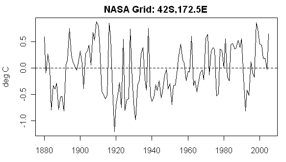
The gridded histories for this gridcell from CRU and NASA are shown below:
wellin66.gif

wellin65.gif

Climate Insensitivity and AR(1) Models

Tamino’s guest post at RC deals with global mean temperature and AR(1) processes. AR(1) is actually mentioned very often in climate science literature, see for example its use in the Mann corpus (refs (1,2,3,4). Almost as often something goes wrong (5,6,7). But this time we have something very special, as Tamino agrees at realclimate that AR(1) is an incorrect model:

The conclusion is inescapable, that global temperature cannot be adequately modeled as a linear trend plus AR(1) process.

This conclusion would be no surprise to Cohn and Lins. But if their view is that global temperature cannot be adequately modeled as a linear trend plus AR1 noise, what are we to make of IPCC AR4, where the caption to Table 3.2 says

Annual averages, with estimates of uncertainties for CRU and HadSST2, were used to estimate. Trends with 5 to 95% confidence intervals and levels of significance (bold: less than 1%; italic, 1 – 5 %) were estimated by Restricted Maximum Likelihood (REML; see Appendix 3.A), which allows for serial correlation (first order autoregression AR1) in the residuals of the data about the linear trend.

This was mentioned here earlier (9). Thus, according to Tamino the time series in question is too complex to be modeled as AR(1)+ linear trend, but IPCC can use that model when computing confidence intervals for the trend!

Continue reading →

World Conference on Research Integrity to Foster Responsible Research

The World Conference on Research Integrity convened in Portugal from 16 to Sept 19. They refer to two incidents – the misrepresentation of the examination of station history in China and the NASA Y2K problem:

Addressing the urgent need for fighting fraud, forgery and plagiarism in science world-wide, the very first World Conference on Research Integrity is set to facilitate an unprecedented global effort to foster responsible research in Lisbon, Portugal from 16 to 19 September 2007.

The controversies surrounding the recent assessment report of the United Nations’ Intergovernmental Panel on Climate Change demonstrates how research integrity is a critical issue not only for the science community, but for politicians and the society as a whole as well. In August 2007 the US National Aeronautics and Space Administration (NASA) had to withdraw previous published historical climate data. The incident came after a British mathematician discovered that the sources used by the Intergovernmental Panel for Climate Change (IPCC) have disregarded the positions of weather stations, plus intentionally using outdated data on China from 1991 and ignoring revised data on the country from 1997.

Now 350 concerned scientists, scientific managers and magazine editors from around the world are scheduled to attend the event in Lisbon, initiated and organised by the European Science Foundation (ESF) and the US Office for Research Integrity (ORI). It marks a milestone for the science community as it will link all those concerned parties in a global effort to tackle the issue head on.
”At the very least, countries should know how misconduct will be handled in other countries and whom to contact if they have questions. A more ambitious goal is to begin to harmonize global policies relating to research integrity,” says Conference Co-Chair Nicholas Steneck from the University of Michigan.

These two issues were both raised at climateaudit. The Chinese station issue was discussed at climateaudit last February here where I said:

Jones et al 1990 described their QC procedures as follows:

“The stations were selected on the basis of station history; we selected those with few, if any changes in instrumentation, location or observation times.

In this case, I have been able to track down third-party documentation on stations used in Jones’ China network and it is impossible that Jones et al could have carried out the claimed QC procedures.

Doug Keenan’s note on this refers to climateaudit initially raising the issue.

The problem with Jones et al. and Wang et al. was first raised on the ClimateAudit blog of Stephen McIntyre (who exposed the “hockey stick” graph of temperatures over the past millennium). McIntyre noted that the stated claims about Chinese data seemed “absurd”. Indeed, for anyone familiar with Mao’s Great Leap Forward and the Cultural Revolution, the claim to have obtained substantial reliable data for 1954–1983 makes little sense.

My initial note went further, observing the inconsistency between the station history information said to be available in the CDIAC Technical Report and the claims in Jones et al 1990. Doug Keenan’s further investigation indicated that co-author Wang was probably responsible. Allocation of fault between the coauthors was a secondary issue as far as I was concerned – the more important issue, in my opinion, being the misrepresentation in Jones et al 1990 that the station histories had been examined. Be that as it may, the identification of the problem with the false claims in Jones et al 1990 to have examined Chinese station history, as Doug acknowledged in his note.

Obviously the identification of the NASA data problem originated here as well. The conference communique has mixed up these rather different issues – something that might have been avoided had they invited people who were familiar with the details of these issues to the conference.

If these issues were on their mind in publicizing the conference, you’d think that they’d have included a presentation on these issues at some point in the 4 days of the proceedings and that they’d have correctly identified the person who identified these errors as Canadian.

Titusville

It’s been awhile since I have shown new USHCN stations, and its not for lack of material. But I got busy with the UCAR conference, publishing a slide show, and other things. But this morning, über volunteer Don Kostuch sent me a note on his latest survey in Titusville, FL near Cape Canaveral and KSC. I’d like to point out that Don has traveled further and surveyed more stations in the USA than anyone. He is a surveying machine. He wrote this in his email to me:

“On your scale of 1 to 5, this is an 8. Peace, Don Kostuch”

Ok in the past we have seen stations on rooftops, at sewage treatment plants, over concrete, next to air conditioners, next to diesel generators, with nearby parking, excessive nighttime humidity, and at non-standard observing heights.

Imagine a USHCN station that embraces all of that. I give you the Titusville, FL USHCN station:

Ever thorough, Don also provided photographs of the Climate Reference Network site, just 7 miles east at KSC, which demonstrates the correct environment for measurement of near surface air temperature:

Now I know there will be the usual critics who will jump in and say “This can be adjusted for!”. Ok here is your chance, show me the equations to untangle Titusville’s temperature record from microsite bias. Personally, it looks FUBAR to me.

"Miscalculation, poor study design or self-serving data analysis"

Dr. Ioannidis, an epidemiologist who studies research methods at the University of Ioannina School of Medicine in Greece and Tufts University in Medford, Mass, has documented how, in thousands of peer-reviewed research papers published every year, there may be so much less than meets the eye. He writes in the WSJ as follows:

Most Science Studies Appear to Be Tainted By Sloppy Analysis

We all make mistakes and, if you believe medical scholar John Ioannidis, scientists make more than their fair share. By his calculations, most published research findings are wrong. …

These flawed findings, for the most part, stem not from fraud or formal misconduct, but from more mundane misbehavior: miscalculation, poor study design or self-serving data analysis. “There is an increasing concern that in modern research, false findings may be the majority or even the vast majority of published research claims,” Dr. Ioannidis said. “A new claim about a research finding is more likely to be false than true..

The hotter the field of research the more likely its published findings should be viewed skeptically, he determined.

Sounds to me like he’d support checking for “miscalculation, poor study design or self-serving data analysis” in climate science as well.

Hansen Step 1

Hansen “Step 1” which was the source of the August crossword puzzles does not occur in a crossword puzzle form in the USHCN stations that we’ve been discussing this week. The “Hansen bias” in combining scribal versions, noticed by John Goetz, does not occur in USHCN stations for two separate reasons: (1) in the USHCN stations that I’ve examined, there is only one dset=0 version and the dset=1 version is equal to the dset=0 version and the “Hansen bias” issue noticed in the Russian stations doesn’t come into play; (2) to be material, the “Hansen bias” requires a very short overlap between the historical data and the MCDW data. For the Russian stations, this is typically only 4 years so that the December 1986 anomaly problem comes into play.

Jean S, as so often, was the first to figure out how the Hansen bias is implemented in multiple versions. He sent me his Matlab code about 2 weeks ago. Since then Hansen has archived his Step 1 code. I’ve done it my own way in R and am compatible with Jean S’ results up to an annoying rounding difference, that should be resolvable.

Jean S code (Matlab) is here
My code (R) is here.

Here are notes on the process. Continue reading →

Should NASA climate accountants adhere to GAAP?

Shortly after, NASA published their source code on Sept 7, we started noticing puzzling discrepancies in the new data set. On Sep 12, 2007, I inquired about the changes to Hansen and Ruedy, observing that there was no notice of the apparent changes at their website:

Dear Sirs, I notice that you’ve changed the historical data for some US stations since Sep 7, 2007. In particular, I noticed that temperatures for Detroit Lakes MN in the early part of the century were reduced by nearly 0.5 deg C. These changes are subsequent to your changes in August 2007 for the changing versions. To my knowledge, there is no explanation for this most recent change and I was wondering what the reason is.


Figure 1. Difference between Sep 10, 2007 version of Detroit Lakes MN and Aug 25, 2007 version.

Thank you for your attention, Steve McIntyre

I posted on the topic on Sept 13 observing:

Since August 1, 2007, NASA has had 3 substantially different online versions of their 1221 USHCN stations (1221 in total.) The third and most recent version was slipped in without any announcement or notice in the last few days – subsequent to their code being placed online on Sept 7, 2007. (I can vouch for this as I completed a scrape of the dset=1 dataset in the early afternoon of Sept 7.)

The impact of the unreported changes was illustrated at Detroit Lakes MN using the same graphic as sent to Hansen and Ruedy. The post included the following prediction:

As you can see, Hansen has clawed back most of the gains of the 1930s relative to recent years – perhaps leading eventually to a re-discovery of 1998 as the warmest U.S. year of the 20th century.

This prediction came true quite quickly. On Sept 15, Jerry Brennan observed that the NASA U.S. temperature history had changed and that 1998 was now co-leader atop the U.S. leaderboard.

By this time, we’d figured out exactly what Hansen had done: they’d switched from using the SHAP version – which had been what they’d used for the past decade or so – to the FILNET version. The impact at Detroit Lakes was relatively large – which was why we’d noticed it, but in the network as a whole the impact of the change was to increase the trend slightly – enough obviously to make a difference between 1934 and 1998 – even though this supposedly was of no interest to anyone.

update42.gif
Average Impact of changing from SHAP to FILNET accounting.

Later on Sept 15, I observed:

This new leaderboard is really something else. I’m going to post on this: but if the SHAP version was what they used for the past decade, it’s a little – shall we say – “convenient” to decide in Sept 2007 that they are going to switch to the FILNET version (without announcing it on their website) and then, surprise, surprise, 1998 is now tied for the warmest year. This is going to send shivers up the spine of any readers familiar with accounting principles.

I’d been planning to write a post on this. There are undoubtedly more Climate Audit readers familiar with GAAP (Generally Accepted Accounting Principles) than at other climate websites, but it’s worth re-stating one of the fundamental GAAP principles:

Principle of the permanence of methods: This principle aims at allowing the coherence and comparison of the financial information published by the company.

Now you may say that this is “science” and accounting principles don’t apply. And my response would be that I’d expect GAAP principles to be a minimum standard for the type of climate statistics being carried out by NASA. Even if NASA climate statisticians are unaware of GAAP per se, they should be adhering to the principles. Sharp practice is sharp practice, however it is gussied up.

Hansen said that the difference between 1998 and 1934 was “statistically insignificant”. But business accountants are familiar with situations where a lot of attention is paid to numbers that may be “statistically insignificant”. I’ll give you an example. For a large corporation, the difference between a small profit and a small loss can be “statistically insignificant”, but there is a big difference in how they are perceived by the public. In some cases, unscrupulous corporations (and you can think of a few, including the most famous recent U.S. bankruptcy) will do whatever they can in terms of deferring expenses or recognizing revenue to change a reported loss into a reported profit. Accounting changes are a red flag to analysts for brokerage companies; there may be “good” reasons but the analyst needs to be right on top of the situation and they will be VERY unimpressed if a company tries to slip a change in without reporting it.

So while the difference between 1934 and 1998 may have been “statistically insignificant”. Hansen was obviously quite annoyed by the attention paid to 1934 being called the “warmest year” even in the U.S. and the change in rankings must have stuck in his craw. Was that motivation in the change from SHAP to FILNET accounting? I certainly hope not. Perhaps long before the Y2K error re-arranged things, NASA had already made long-standing plan to shift from SHAP accounting to FILNET accounting. But if this was not the case, then the timing of the change, especially with the all too “convenient” restoration of 1998 to the top of the leaderboard is certainly unfortunate.

This is precisely the type of situation that would have been avoided by NASA adhering to GAAP principles. Companies cannot change accounting procedures on a whim. Auditors will not permit companies to change methods merely to enhance reported earnings. And if a company changed accounting procedures without any disclosure, it would be viewed very seriously by regulatory agencies – whether or not the company said that it “mattered”. If the change from SHAP to FILNET accounting didn’t “matter”, then Hansen shouldn’t have done it. If it did matter, he still shouldn’t have done it right now just when he was archiving source code for the first time – and to do so without either formal disclosure or a re-statement of prior results simply boggles the imagination.

On Sept 17, Ruedy replied to my email asking that they disclose their changes, more or less refusing on the basis that the new data source could be detected in the “description of input files” in the source code.

Dear Sir,
As indicated in the description of our input files, we switched from the old year 2000 version of USHCN to the current version. The differences you noticed reflect corrections that were made by USHCN within the last six years.
Reto A. Ruedy

But this is not the same as a change statement. There’s no hint in the input file itself that they had changed the input file from what had been used previously and that the code archived on Sept 7 was NOT the code used to produce NASA results prior to Sept 7. They had not merely “simplified” the code; they had changed from SHAP to FILNET accounting. It’s also not good enough to simply slip the accounting change in with the source code. It should have been formally disclosed when the change was instituted, rather than leaving us to try to figure it out and (later disclosing it only when the change had already been discovered.)

In addition, his last sentence here – that the changes “reflect corrections that were made by USHCN within the last six years” is not correct. Both SHAP and FILNET accounts existed when Hansen et al 2001 was written. Hansen decided – for whatever reason- to use SHAP accounting. HE could have used FILNET accounting. And he decided to change in mid-September 2007. Did it “matter”? Well, it mattered enough to go to the trouble of making the change. It also – and perhaps this is sheer coincidence – mattered to the “statistically insignificant” leaderboard as 1998 is now your new co-leader/

Today NASA has attempted to cooper up this mess. At their website, they finally reported the change in accounting that we had already picked up and reported. They state:

September 2007: The year 2000 version of USHCN data was replaced by the current version (with data through 2005). In this newer version, NOAA removed or corrected a number of station records before year 2000. Since these changes included most of the records that failed our quality control checks, we no longer remove any USHCN records. The effect of station removal on analyzed global temperature is very small, as shown by graphs and maps available here.

This seems like a pretty odd description of what they appear to have done and perhaps I’ll re-visit this on another occasion. Hansen includes the following account of the Y2K error (conspicuously deleting his prior recognition of my role in identifying the error) and adding a reference to Usufruct and the Gorilla at the NASA website:

August 2007: A discontinuity in station records in the U.S. was discovered and corrected (GHCN data for 2000 and later years were inadvertently appended to USHCN data for prior years without including the adjustments at these stations that had been defined by the NOAA National Climate Data Center). This had a small impact on the U.S. average temperature, about 0.15’C, for 2000 and later years, and a negligible effect on global temperature, as is shown here.

This August 2007 change received international attention via discussions on various blogs and repetition by some other media, with no graphs provided to show the magnitude of the effect. Further discussions of the curious misinformation are provided by Dr. Hansen on his personal webpage (e.g., his post on “The Real Deal: Usufruct & the Gorilla”).

Obviously his claim that “no graphs had been provided to show the magnitude of the effect” is false. In one of my original posts on the matter, I showed graphics estimating the impact of the error on the U.S. temperature record and the distribution of errors on USHCN stations. I sent the following letter to Hansen and Ruedy today, notifying them that his statement was incorrect as follows:

Dear Sirs,

I see that you have decided to report the change in methodology as requested in my previous email. While you should have reported the change in methodology when it was made, it is better late than never.

In your new webpage, you state: ” This August 2007 change received international attention via discussions on various blogs and repetition by some other media, with no graphs provided to show the magnitude of the effect.” This is incorrect and I request that you correct this statement. On Aug 6, 2007, at Climate Audit, http://www.climateaudit.org/?p=1868 , the two graphs below were provided to estimate the magnitude of the effect. The first graph shown below estimated the impact on the U.S. temperature history at a little more than 0.15 deg C. Despite having no access to your source code, this proved to be an accurate estimate.

The next graph shown below shows the distribution of changes over the 1221 U.S. stations, which are very substantial in individual cases. Despite your professed concern for illustrating the impact of changes, you did not yourself provide any graph to show the magnitude of the changes on individual stations, nor did you even provide explicit notice on your webpage that any changes had been made.

Would you please correct the incorrect information on your webpage. This request is made pursuant to the Data Quality Act.

Yours truly,
Stephen McIntyre

A last point: as I’ve noted previously, as the classification of U.S. sites comes in, the actual GISS methodology for estimating U.S. temperatures looks a lot better than (say) the NOAA methodology. If NASA’s U.S. estimates stand up to scrutiny, that’s fine: that wouldn’t bother me a speck. I’m just trying to understand what weight can be put on which estimates. And regardless of what people may think, in a quick review of my posts, I haven’t located any posts in which I am particularly critical of NASA’s methods in the U.S., aside from the Y2K error. My position has been more: if NASA’s adjustments are right, then Parker 2006 and Jones et al 1990 etc are wrong. I had not personally criticized their lights methodology for classifying stations, preferring to see how station evaluation turned out. I have criticised poor and inaccurate disclosure, some of Hansen’s public comments and surveyed some of the data issues in the ROW (where’s Waldo?).

But I don’t think that I’ve been particularly critical of their U.S. methodology and, if the lights on-lights off criterion is a useful one for urban adjustments, that’s fine with me and I’ll be happy to acknowledge it. As noted elsewhere, that would leave many other open questions pertaining to the ROW, why there are discrepancies between NASA and NOAA, why NASA overall results are so similar to CRU results, if the individual stations are adjusted so differently etc etc.

But these matters are all quite different than (a) changing accounting systems; (b) doing so without notice; (c) archiving source code where the input file had been changed from what had been previously used; (d) making false statements on a NASA website.

UPDATE Sept 17 afternoon: Ruedy responded to my email as follows:

Thanks for bringing to our attention that the term “magnitude of effect” might be interpreted as “size” rather than “relevance”, our obvious intent. We clarified our formulation correspondingly.

They changed their website to read as follows (replacing magnitude with relevance):

This August 2007 change received international attention via discussions on various blogs and repetition by some other media, with no graphs provided to show the relevance of the effect.

Needless to say, this claim remains untrue. I sent the following letter (repeating the graphics shown above) requesting that the webapge be corrected, this time copying the Info Quality person at NASA:

Your revised webpage http://data.giss.nasa.gov/gistemp/ contains the following incorrect statement: “This August 2007 change received international attention via discussions on various blogs and repetition by some other media, with no graphs provided to show the relevance of the effect.”

This is incorrect and I request that you correct this statement. As I advised you previously, on Aug 6, 2007, at Climate Audit, http://www.climateaudit.org/?p=1868 , the two graphs below showed the relevance of the effect to U.S. temperature history and to U.S. stations.

The first graph shown below showed that the error was relevant to U.S. temperature history – a topic specifically considered in Hansen et al 2001.

The NASA website provides individual station histories, as well as U.S. and global estimates. The graph below showed the error was relevant to individual U.S. station histories.

The claim that “no graphs provided to show the relevance of the effect” remains incorrect. Once again, please correct the false statement on the NASA webpage http://data.giss.nasa.gov/gistemp/ . This request is made under the Data Quality Act.

Yours truly,
Steve McIntyre
A Second Look at USHCN Classification

Yesterday, I posted up a first look at differences between station histories classified as CRN=1 (good) versus CRN=5 (bad) – a simple comparison of averages, noting that other factors may well enter into the comparison.

A couple of other points that I’ve made consistently as we look at these results which I’d like people to keep in mind:

(1) the elephant in the room in these station studies is the difference in trends between the US history with 1930s at levels more or less similar to the 2000s and the ROW with a pronounced trend (where’s Waldo?);

(2) the US network has a large representation of rural stations which have records stretching back to the 1930s, a different situation than for the ROW;

(3) NOAA and NASA have quite different procedures, with NOAA showing a much more pronounced trend than NASA in the US 48

(4) whatever the warts on the NASA methodology, they at least make a more concerted effort to adjust for urbanization in their U.S. network (relative to NOAA) and we need to keep both networks in mind. In particular, NASA already has a high 1934 relative to 1998, especially as compared to NOAA.

While NASA has been taking the brunt of recent criticism, it is actually NOAA rather than NASA that has made highly publicized announcements about 2006 being the “warmest year” and we need to keep this in mind as our understanding of these methods and data improves.

Continue reading →

Is Juckes et al 2006 Peer Reviewed?

As readers of this blog know, Juckes et al submitted a paper for online review at Climate of the Past Discussions. See here for discussion. There were many unsatisfactory and even distasteful aspects to this paper. I submitted a detailed online review, as did Willis Eschenbach and another CA reader. I spent time rebutting a variety of unsupportable allegations about our paper. I did so in the belief that the online review process at CPD was a bona fide process. It appears that this belief was mistaken.

The responsible editor, H. Goosse, was a serial coauthor with Michael Mann and not particularly well-disposed towards the MM criticisms of MBH. Although I was an invited reviewer of B’rger’s re-submission, Goosse made no reference to either my review or to Willis’ review in his comments to Juckes et al. However, he did indirectly call for Juckes et al to “strongly reduce” their section purporting to criticize us and only “briefly” mention this controversy:

One exception is section 3 “critic of the IPCC2001 consensus on millennial temperatures”. This part is devoted to a very specific topic, difficult to follow for readers who are not familiar with previous work and to my point of view is not clearly connected to the other parts of the manuscript even in the revised version. This section is already long compared to the other ones of the manuscript, although some parts would require some more detailed information. I consider thus, at this stage, that this discussion should be much clearer if this was let that to another paper or note specifically devoted to this subject. In agreement with the Referee, I would thus recommend that the authors strongly reduce this section and briefly mention the controversy about the “IPCC2001 consensus” in section 2.

So while Goosse was undoubtedly not inclined to do us any favors, he clearly did not accept the Juckes submission. B’rger went to a considerable effort to re-submit a CPD submission and I guess that most of us assumed that Juckes et al would re-submit, just as B’rger had to re-submit.

However, we’ve seen no re-submissions. However, if you look at the references for Ammann and Wahl 2007, you will see:

Juckes MN, Allen MR, Briffa KR, Esper J, Hegerl GC, Moberg A, Osborn TJ, Weber SL, Zorita E (2006) Millennial temperature reconstruction intercomparison and evaluation. Clim Past Discuss 2:1001’1049

So Juckes et al don’t seem to have bothered going to the trouble of re-writing to meet referee comments. But it’s still cited in a Climatic Change article as though it was peer reviewed. We’ve seen examples in the Ammann/Mann corpus of academic check kiting. Surely this is a case of review avoidance if not actual review evasion (borrowing the terminology from tax law.)

And surely this is damaging to the reputation of Climate of the Past and should be protested by its editors. The CP experiment was an experiment in online and open peer review. CP Discussion editors had minimal requirements for posting online, presumably on the basis that online review comments would be taken seriously by authors. Ammann, Wahl, Juckes, Allen, Esper, Hegerl, Moberg, Osborn, Weber and Zorita have demonstrated a total disregard for the CP process by citing (and allowing their article to be cited) even though CP editors had asked that changes be made. And now Climatic Change has acquiesced in this continuing degradation of the currency by permitting Juckes et al 2006 to be cited as though it were a peer reviewed article.

Time for Climate of the Past editors to speak up.