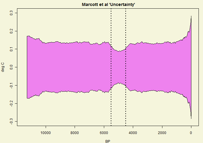
So far, the focus of the discussion of the Marcott et al paper has been on the manipulation of core dates and their effect on the uptick at the recent end of the reconstruction. Apologists such as “Racehorse” Nick have been treating the earlier portion as a given. The reconstruction shows that mean global temperature stayed pretty much constant varying from one twenty year period to the next by a maximum of .02 degrees for almost 10000 years before starting to oscillate a bit in the 6th century and then with a greater amplitude beginning about 500 years ago. The standard errors of this reconstruction range from a minimum of .09 C (can this set of proxies realistically tell us the mean Temperature more than 5 millennia back within .18 degrees with 95% confidence?) to a maximum of .28 C. So how can they achieve such precision?
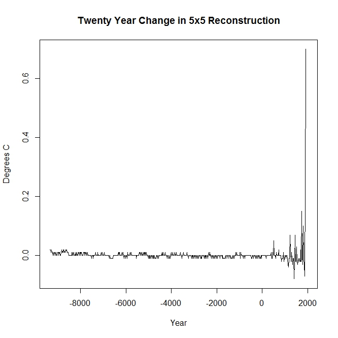
The Marcott reconstruction uses a methodology generally known as Monte Carlo. In this application, they supposedly account for the uncertainty of the proxy by perturbing both the temperature indicated by each proxy value as well as the published time of observation. For each proxy sequence, the perturbed values are then made into a continuous series by “connecting the dots” with straight lines (you don’t suppose that this might smooth each series considerably?) and the results from this are recorded for the proxy at 20 year intervals. In this way, they create 1000 gridded replications of each of their 73 original proxies. This is followed up with recalculating all of the “temperatures” as anomalies over a specific 1000 period (where do you think you might see a standard error of .09?). Each of the 1000 sets of 73 gridded anomalies is then averaged to form 1000 individual “reconstructions”. The latter can be combined in various ways and from this set the uncertainty estimates will also be calculated.
The issue I would like to look at is how the temperature randomization is carried out for certain classes of proxies. From the Supplementary Information:
Uncertainty
We consider two sources of uncertainty in the paleoclimate data: proxy-to-temperature calibration (which is generally larger than proxy analytical reproducibility) and age uncertainty. We combined both types of uncertainty while generating 1000 Monte Carlo realizations of each record.
Proxy temperature calibrations were varied in normal distributions defined by their 1σ uncertainty. Added noise was not autocorrelated either temporally or spatially.
a. Mg/Ca from Planktonic Foraminifera – The form of the Mg/Ca-based temperature proxy is either exponential or linear:
Mg/Ca = (B±b)*exp((A±a)*T)
Mg/Ca =(B±b)*T – (A±a)
where T=temperature.
For each Mg/Ca record we applied the calibration that was used by the original authors. The uncertainty was added to the “A” and “B” coefficients (1σ “a” and “b”) following a random draw from a normal distribution.
b. UK’37 from Alkenones – We applied the calibration of Müller et al. (3) and its uncertainties of slope and intercept.
UK’37 = T*(0.033 ± 0.0001) + (0.044 ± 0.016)
These two proxy types account for (19 (Mg/Ca) and 31 (UK’37)) 68% of the proxies used by Marcott et al. Any missteps in how these are processed would have a very substantial effect on the calculated reconstructions and error bounds. Both of them use the same type of temperature randomization so we will examine only the Alkenone series in detail.
The methodology for converting proxy values to temperature comes from a (paywalled) paper: P. J. Müller, G. Kirst, G. Ruthland, I. von Storch, A. Rosell-Melé, Calibration of the alkenone 497 paleotemperature index UK’37 based on core-tops from the eastern South Atlantic and the 498 global ocean (60N-60S). Geochimica et Cosmochimica Acta 62, 1757 (1998). Some information on Alkenones can be found here.
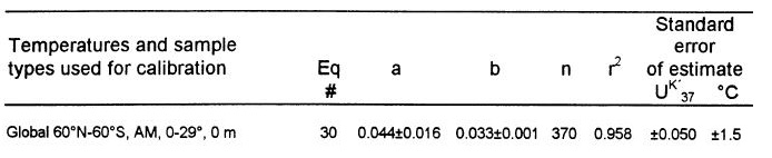
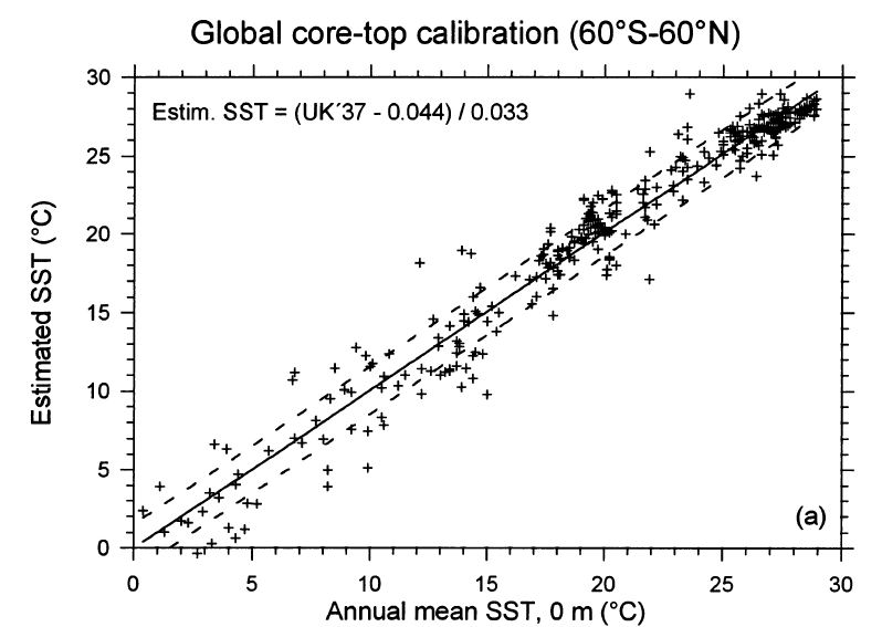
Müller et al use simple regression to derive a single linear function for “predicting” proxy values from the sea surface temperature:
UK’37 = (0.044 ± 0.016) + (0.033 ± 0.001)* Temp
The first number in each pair of parentheses is the coefficient value, the second is the standard error of that coefficient. You may notice that the standard error for the slope of the line in the Marcott SI is in error (presumably typographical) by a factor of 10. These standard errors have been calculated from the Müller proxy fitting process and are independent of the Alkenone proxies used by Marcott (except possibly by accident if some of the same proxies have also been used by Marcott). The relatively low standard errors (particularly of the slope) are due to the large number of proxies used in deriving the equation.
According to the printed description in the SI, the equation is applied as follows to create a perturbed temperature value:
UK’37 = (0.044 + A) + (0.033 + B)* Pert(Temp)
[Update: It has been pointed by faustusnotes at Tamino’s Open mind that certain values that I had mistakenly interpreted as standard errors were instead 95% confidence limits. The changes in the calculations below reflect the fact the the correct standard deviations are approximate half of those amounts: 0.008 and 0.0005.]
where A and B are random normal variates generated from independent normal distributions with standard deviations of 0.016 0.008 and 0.001 0.0005, respectively.
Inverting the equation to solve for the perturbed temperature gives
Pert(Temp) = (UK’37 – 0.044)/(0.033 + B) – A / (0.033 + B)
If we ignore the effect of B (which in most cases would have a magnitude no greater than .003), we see that the end result is to shift the previously calculated temperature by a randomly generated normal variate with mean 0 and standard deviation equal to 0.016/0.033 = .48 0.008/0.033 = 0.24. In more than 99% of the cases this shift will be less than 3 SDs or about 1.5 0.72 degrees.
So what can be wrong with this? Well, suppose that Müller had used an even larger set of proxies for determining the calibration equation, so large that both of the coefficient standard errors became negligible. In that case, this procedure would produce an amount of temperature shift that would be virtually zero for every proxy value in every Alkenone sequence. If there was no time perturbation, we would end up with 1000 almost identical replications of each of the Alkenone time series. The error bar contribution from the Alkenones would spuriously shrink towards zero as well.
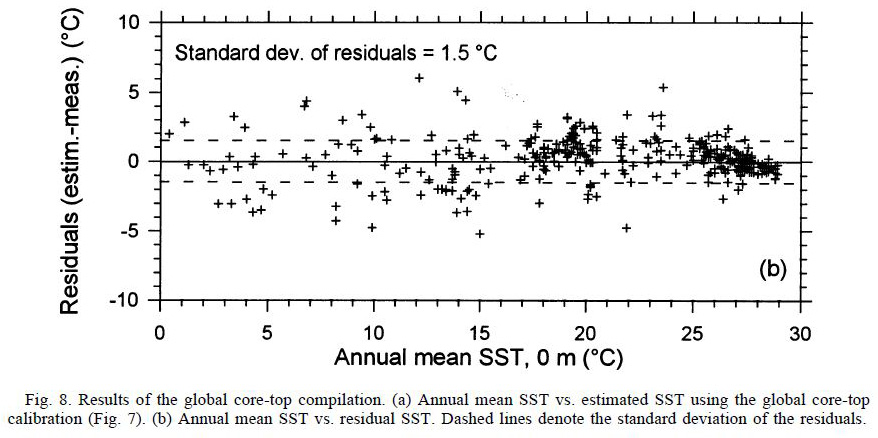
What Marcott does not seem to realize is that their perturbation methodology left out the most important uncertainty element in the entire process. The regression equation is not an exact predictor of the the proxy value. It merely represents the mean value of all proxies at a given temperature. Even if the coefficients were known exactly, the variation of the individual proxy around that mean would still produce uncertainty in its use. The randomization equation that they should be starting with is somewhat different:
UK’37 = (0.044 + A) + (0.033 + B)* Pert(Temp) + E
where E is also a random variable independent of A and B and with standard deviation of the predicted proxy equal to 0.050 obtained from the regression in Müller:
The perturbed temperature now becomes
Pert(Temp) = (UK’37 – 0.044)/(0.033 + B) – (A + E) / (0.033 + B)
and again ignoring the effect of B, the new result is equivalent to shifting the temperature by a single randomly generated normal variate with mean 0 and standard deviation given by
SD = sqrt( (0.016/0.033)2 + (0.050/0.033)2 ) = 1.59
SD = sqrt( (0.008/0.033)2 + (0.050/0.033)2 ) = 1.53
The variability of the perturbation is now three 6.24 times as large as that calculated when only the uncertainties in the equation coefficients are taken into account. Because of this, the error bars would increase substantially as well. The same problem would occur for the Mg/Ca proxies as well, although the magnitudes of the increase in variability would be different. In my opinion, this is a possible problem that needs to be addressed by the authors of the paper.
The regression plot and the residual plot from Müller give an interesting view of what the relationship looks like.
I would also like someone to tell me if the description for ice cores means what I think it means:
f. Ice core – We conservatively assumed an uncertainty of ±30% of the temperature anomaly (1σ).
If so, …
 ]
]

 Bobbie Hasselbring, editor of Real Food Traveller, has an article on “Aging as a State of Mind”. Her