How Al Gore Saved Christmas

Obviously it’s impossible to avoid the old chestnuts on our TV sets these days. I saw the original version of Miracle on 34th St for the umpteenth time the other day, noticing something for the first time that is a sign of the times. The judge’s political handler, advising him of the political risks of the case, warned him that a decision against Kris Kringle would draw the ire of toy-makers, all unionized and all voters. How quaint.

It’s also impossible to avoid the snow. We got hit with another snow storm yesterday and, for the first time in my life, I was pondering whether I should be thinking about planning my snow banks so that I’d have a place for the snow later in the season. (Through my life, it’s never been an issue in Toronto, we don’t get that much snow as we’re in a bit of a shadow and what we get tends to come and go.) But last year we had snow banks into April and it became hard to figure out where to put the snow.

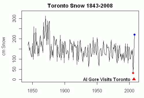
While thinking about this, I pondered about how Al Gore saved Christmas for us in Toronto, a story that’s been told before, but it’s the season for old stories.

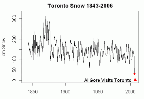
Long ago (2006), in the bad old days before IPCC AR4, Toronto got its lowest snowfall in a century. Lake level declines were sure to follow. Would water supplies for lattes be threatened? Even the unthinkable now seemed possible and even likely.

Nobody knew what do. Except for one little girl. (Hey, it’s a story.) She wrote to a famous ju-ju man in the South asking him to come north and cast a magic spell and make the snow return.

The ju-ju man heard the plea of the little girl. He quickly decided that the situation was far worse than even the little girl thought. This needed his most powerful magic and, so in 2007, he visited Toronto not just once, not just twice but three times.

The magic worked! Soon Toronto was covered up in winter snow. The ju-ju man could only save part of the 2007 winter, but by 2008, his magic was in full force. Yesterday’s snow made 2008 snowfall the highest since 1883, with a few days still on the clock.

And it was all due to that one little girl.

As for me, my arms ache from shoveling snow. I think that the ju-ju man might overdid his spell a little. I’d have been OK with just one incantation.

2008

Merry Christmas to all of you. And to Mike, Gavin, Jim, Ben and and all those who have worked so hard to provide us with interesting statistical entertainment during the past year.

Downloading KNMI Model Data

Lucia has been experimenting with model data downloaded from KNMI and I thought that I’d try to experiment with this a little from time to time.

Unlike Benjamin Santer, Ph.D. of the U.S. federal Lawrence Livermore Labs, who refused to provide any assistance whatever in providing the data used in Santer et al, Geert Oldenburgh, the KNMI scientist responsible for their public interface, is pleasant and cooperative though it seems that they aren’t used to automated data inquiry of the type that I expect to do.

Their webpage is designed for manual retrieval, but it can be pinged so that data can be directly downloaded into R. KNMI had no objections to me trying to do this and Oldenburgh helped as much as he could. I’ve managed to write a neat little retrieval script that picks up ensemble combinations but I’m stumped as to how to retrieve individual runs. It looks like it should be possible; KNMI has no objection to my doing so; maybe one of the computer-oriented readers can solve this little puzzle.

Here’s what I can do so far.

The access point are cgi commands in the URL that instruct the KNMI computer to compile averages. This works very quickly. Examples of these commands are:

http://climexp.knmi.nl/get_index.cgi?email=yourname@you&field=tas_bcc_cm1_20c3m&standardunits=true

or

http://climexp.knmi.nl/get_index.cgi?email=yourname@you&field=tas_bcc_cm1_20c3m&standardunits=true&lat1=-20&lat2=20&lon1=0&lon2=360

If you insert this sort of URL in your browser, it will ping the KNMI computer to produce ensemble temperature averages for the region specified by the lat-long (default – global.) The HTML page that is produced contains information on the location of the sought data file. The information can be grep’ed from the HTML page and a new URL can be constructed where the ensemble average is located. This file can be read fairly easily – there’s an annoying comment at the end of the file that requires extra handling, but this is programmed easily enough. I’ve inserted the program below.

The ensemble averages is fine. Here’s where I get stuck on reading individual runs. Go to http://climexp.knmi.nl and then ping Scenario Runs on the right frame under Select A Field. Now as an example, check the radio button under tas for BCC_CM1 and click Select Field.

If you click Make Time Series in the first panel, this will make the ensemble average, producing a new page. Above the third panel in the new page is a hyperlink “raw data” which contains a time series of anomaly data. This is what I can retrieve with the script below.

If you now go back to the previous page, you’ll see hyperlinks at the bottom of the page which produce results from each of two different runs. If you click the hyperlink of “analyse ensemble member 1 separately”, it will generate a webpage looking just like the one we just had, except this time if you click Make Time Series in the first panel, it produces the results of this run located in a webpage structured as before.

I presume that there is a cgi command generated by one of these links, but I haven;t been able to figure out the structure. Maybe one of the computer programmers who visits here can figure it out.

Here are my scripts. Please paste in a real email address in the appropriate spot below (requested by Oldenburgh) so that usage of the access tools can be reported.

##FUNCTIONS
read.ensemble=function(model,scenario,prefix=myprefix,region=”GL”,suffix= “&standardunits=true”) {
if (region==”TRP”) {suffix=”&standardunits=true&lat1=-20&lat2=20&lon1=0&lon2=360″;suffix2=”0-360E_-20-20N”}
if (region==”NH”) {suffix=”&standardunits=true&lat1=0&lat2=90″;suffix2=”0-360E_0-90N”}
if (region==”SH”) {suffix=”&standardunits=true&lat1=-90&lat2=0″;suffix2=”0-360E_-90-0N”}
if (region==”arctic”) {suffix=”&standardunits=true&lat1=60&lat2=90″;suffix2=”0-360E_60-90N”}
if (region==”antarctic”) {suffix=”&standardunits=true&lat1=-90&lat2=60″;suffix2=”0-360E_-90-60N”}
if (region==”GL”) {suffix=”&standardunits=true”;suffix2=”0-360E_-90-90N”}

url=paste(paste(prefix,model,scenario,sep=”_”),suffix,sep=””)
#http://climexp.knmi.nl/get_index.cgi?email=yourname@you&field=tas_bcc_cm1_20c3m&standardunits=true
# “http://climexp.knmi.nl/get_index.cgi?email=yourname@you&field=tas_bcc_cm1_20c3m&standardunits=true&lat1=-20&lat2=20&lon1=0&lon2=360”
my_info=download_html(url)
grep(“raw data”,my_info)
y= my_info[grep(“raw data”,my_info)][3]
# “raw data, ”
n=nchar(y)
loc=file.path(“http://climexp.knmi.nl”,substr(y,10,n-16))
Sys.sleep(2)
test=readLines(loc)
count=as.numeric(substr(test[1],19,26))+1
writeLines(substr(test[3:length(test)],1,20),”temp.dat”)
test=read.table(“temp.dat”);
x=test[1,1];x
read.ensemble=ts(test[,2],start= c(floor(x),round( 12* (x%%1),0)+1),freq=12)
read.ensemble}

download_html =function(url) {
download.file(url, “temp.html”);
html_handle < – file(“temp.html”, “rt”);
html_data <- readLines(html_handle);
close(html_handle);
unlink(“temp.html”);
return(html_data);
}

Here is a sample use. This can easily be modified for bulk retrieval.

knmi.info=read.csv(“http://data.climateaudit.org/data/models/knmi.info.csv&#8221;,sep=”\t”)
scenario=”20c3m”
temp=(knmi.info$scenario==scenario);sum(temp) #24
id=unique(knmi.info$alias[temp]);K=length(id) #24
email=”yourname@you” #
myprefix=paste(“http://climexp.knmi.nl/get_index.cgi?email=&#8221;,email,”&field=tas”,sep=””)
i=1; test=read.ensemble(model=id[i],scenario,region=”GL”));

Minus 60 (deg C)?

One of the interesting by-products of the GISS screw-up in October was that we learned the names and locations of quite a few Siberian weather stations – that are glaring “hot spots” on temperature anomaly maps. However, most of these places are among the coldest places on earth.

One of them was Verhojansk, about which Anthony Watts had an interesting post last week; it was one of the screwed up NOAA-Hansen sites. It vies for the title of coldest place (in the Northern Hemisphere) with nearby Ojmjakon.

I’ve taken to occasionally checking on these sites to see how they’re doing and there’s something interesting to watch for over the next few days – the sort of thing that might appeal to people who liked following the summer ice melt. Daily weather information for Ojkjakon is online here

Anyway, in the GHCND history for Ojmjakon online here , there hasn’t been a minus 60 deg C day in December for 15 years and only one in the past 25 years. There has been only one December temperature at Ojmjakon below 62.5 in the GHCND archive (since 1943) – a reading of -62.8 in 1984.

But according to the forecasts here, a low of minus 60 is forecast tonight and minus 63 tomorrow.

The GHCND daily records are maintained consistently up to 2000, but archiving of daily data became very sporadic following the IPCC TAR report. Over the past week, GHCN-D has not managed to record temperatures that were readily available online.

2008 Tropical Temperatures

The blog world is jump starting discussion of 2008 annual temperatures. Yesterday at 1:56 pm Eastern, NASA employee Gavin Schmidt and climate modeler, purely in his “private” capacity, posted an article arguing that the results were consistent with climate models – an activity that lesser minds might think relates to his employment.

Lucia commented here, perhaps redundantly, that Schmidt’s comment was “tendentious twaddle”.

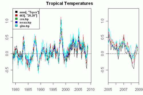
As a result of Ross McKitrick’s “T3” concept (discussed at CA here), I’ve been following tropical [tropospheric] temperatures from time to time, as these are supposed to be “fingerprints” of AGW and decided that it would be timely to update tropical (20S-20N) estimates, using reported satellite data and collating tropical averages from gridded CRU, GISS and NOAA versions as these are not reported separately. I calculated results over the satellite period (1979-2008) for consistency (as I’ve been doing in the past.) In each case, I zero-ed the data over the 1979-1997 period – the choice doesn’t matter much – but I didn’t want to include the most recent period in the normalization period and I wanted a relatively long period. I also divided the satellite temperatures by 1.2 according to a factor sent to me by John Christy. This yielded the following:

Figure 1: Annual Tropical Temperatures. (Centered on 1979-1997)

We now have a 30-year period of satellite records. Within that period, 2008 ranked 26th out of 30 (5th coldest), 23rd for RSS, 16th for CRU and 15th for NOAA and GISS. Tropical temperatures in 2008 were lower in 4 of 5 indices than in 1988, the year of Hansen’s famous testimony.

Although climate scientists downplayed individual cold months early in the year, Schmidt seized on recent Oct and Nov data from GISS:

In GISTEMP both October and November came in quite warm (0.58ºC), the former edging up slightly on last month’s estimate as more data came in.

Figure 2: Monthly Tropical Temperatures. (Centered on 1979-1997)

In the tropics, temperatures in October and November have rebounded from lows early in the year, but GISS is running a bit warmer than the others (about 0.2 deg C relative to the 1979-1997 average).

When I squint at the tropical data, it has two quite different aspects depending on your perspective. On the one hand, you can look at it and conclude that the average level of the cycles is moving up, with the 2008 low being higher than prior lows, with the overall package moving up in an disorderly way. On the other hand, you can look at the data and surmise that it has consistent with 1/f noise or 1/f noise with a very minor trend. It’s hard to believe that this is the sort of result that Gavin Schmidt “wants”.

For people that look at data, it is obvious that the data (in each incarnation) is highly autocorrelated; the degrees of freedom in autocorrelated data can be much lower than people think and, accordingly, the confidence intervals can be surprisingly wide (a point made in Santer et al 2008, though there are some defects in their analysis that we discussed before).

Wide confidence intervals are a two-edged sword. For people who attempt to argue that this data shows no trend, the wide confidence intervals permit a trend much higher than observations (and perhaps high enough to be consistent with the less aggressive models). For modelers who argue (a la Santer) that the confidence intervals are wide (and wide enough so that observations are not “inconsistent” in some sense with models), the problem is that such wide confidence intervals will probably include the null hypothesis of no trend or a minimal trend. It’s interesting to watch, but I don’t think that you can conclude very much either way purely on the statistics of the data, as people so often try to do.

Schmidt observed:

The bottom line: In the GISTEMP, HadCRU and NCDC analyses D-N 2008 were at 0.43, 0.42 and 0.47ºC above the 1951-1980 baseline (respectively). In GISTEMP both October and November came in quite warm (0.58ºC), the former edging up slightly on last month’s estimate as more data came in. This puts 2008 at #9 (or #8) in the yearly rankings, but given the uncertainty in the estimates, the real ranking could be anywhere between #6 or #15

More on Speleothem Dating

I’d like to finish off our discussion of the supposed “strong visible anticorrelation” between the Q5 (Oman) and D1 (Socotra) speleothems (as supposedly evidenced in Figure 9), before discussing millennial issues. Again, I preface these remarks by saying that there is much of interest in speleothems and I’m just discussing one statistical issue here that happened to catch my eye.

As noted before, although I have no wonderful recipes for testing correlation of irregularly sampled series with dating errors, we’ve already seen that, if the Q5 dates were brought about 75 years closer to the present, the sign changed from inverse to positive and the positive correlation was noticeable more “significant” than the weak inverse correlation (correlations being calculated on data interpolated to an annual basis.)

In the 2700-4700BP overlap section under discussion, there were multiple date points for each series. If errors in these date points were independent, then the case for a relatively “stiff” displacement of one series relative to another would be pretty strained; however, it there were something in the method of estimating date that biased one core relative to another, then a relatively “stiff” displacement of Qunf Q5 with respect to Socotra D1 would be a definite possibility.

This led us to examine the dating methods for speleothems – and dating methods are something that interest me. Speleothems are dated using U-Th dating, an interesting technique. Edwards 1987 is a seminal article and I was able to more or less replicate their calculations. U-Th dating calculations work best when there is no native Th in the system – something that is substantially true for the corals that Edwards 1987 was concerned with. As the technique gets extended to other types of data e.g. speleothems, adjustments for Th-230 not arising from the U-238 system needed to be developed.

The Th-232 levels in Q5 are about an order of magnitude higher than in D1. Intuitively, this seems like the sort of place that one would look for potential uncertainties in the calculation that might permit a systemic difference of 75 years. Fleitmann et al 2007 note Th issues and describe their methodology as follows:

In some cases, detritus corrections were needed when 230Th/232Th ratios were high (see Table 1). If necessary, ages were corrected assuming a 232Th/234U ratio of 3.8 (see Frank et al., 2000 for details).

With due respect to Dr Fleitmann, this sort of verbal description occurs all too often in paleoclimate methodology descriptions and shows one more time the benefit of including source code in an SI. What is the benchmark for triggering a “detritus” correction? Why do this for “some” cases and not “all” cases? Issues like this would be instantly clarified by consulting code; in the absence of code, one has to try to guess what the authors did, a pointless and time-consuming exercise, which is one reason why calculations are so seldom verified.

Turning to Frank et al 2000 (online here.) merely compounds the replication problems. Frank et al 2000 nowhere mentions a “232Th/234U ratio of 3.8” so one has to guess.

Frank et al 2000
In addition, Frank et al 2000 is also a practical article on German travertines, where the methodological issue of adjustments is mentioned in passing in an appendix, without providing clear benchmark information to enable one to readily ensure that one is doing the calculations apples-and-apples.

Stepping back for a moment from annoying dating techniques, Frank et al describe interesting geological evidence of the warm period about 110,000 years that was the interglacial prior to the present Holocene. The warmth permitted the growth of travertine around Bad Cannstatt, Germany. Travertine formation ceased during glacial periods and resumed only in the Holocene. U-Th dating is a technique that permits independent dating of the travertine deposits to this period. Frank reported a date of ~105,000 for the laminar Biedermann travertine (which also had leaf imprints of oak, ash, poplar and Mediterranean honeysuckle trees) and several thousand years later (~98-101,000) for the laminar Deckerstrasse travertine.

Frank et al (note to Table 1) report the use of the following equation with Th232-corrected values (and the same decay constants as Edwards 1987):

With a bit of experimenting, this proves to be equivalent to the corresponding equation in Edwards 1987 (multiplied by [U238/U234]_act ).

The Th adjustment deducts an allowance for non-U238-sourced Th-230 using the following equation (Appendix):

This adjustment requires two empirical constants: R_0 is the Th230/Th232 activity of present-day spring water (1.85 -see page 42), used here as an approximation for ancient spring water, while R_d is the Th230/Th232 activity of detritus estimated at 0.526 (based on a sample from a nearby travertine site (Hass/Lauster).

I’ve tried pretty hard to replicate the results in Frank et al 2000 and have got close, but can’t quite replicate them. Without being able to do so, it’s impossible to test the Th-adjustments in Fleitmann et al 2007. For what it’s worth, here is my attempt to replicate the calculations of Frank et al 2000:

First, here are the constants collated from various locations in the paper:

lambda=NULL; lambda[“Th230”]= 9.195E-6#Table 1 Frank
lambda[“U234”]= 2.835E-6 # Table 1
lambda[“U238”]= 1.551E-10 #Table1
R0=1.85;Rd=.526

Next here is the information in Frank Table 1, collated by cut and pasting from the pdf into Notepad and tidying:

A=read.table(“http://data.climateaudit.org/data/speleothem/Frank.2000.edited.dat&#8221;,sep=”\t”,header=TRUE)

Next here is an implementation of the function in Frank et al 2000, combining the equation in the note to Table 1 (the one that corresponds to Edwards 1987 Equation 1) and the Th-adjustment equation in the Appendix.

f=function(t) {
X=act.Th230_U234-act.Th232*(R0-Rd)*exp(-lambda[“Th230”]*t)-act.Th232*Rd #equation A1
B=act.U238_U234* (1-exp(-lambda[“Th230”]*t) )
C= (1- act.U238_U234)* lambda[“Th230”]/(lambda[“Th230”]-lambda[“U234”])
D= (1- exp( -(lambda[“Th230”]-lambda[“U234”])*t) )
f= (X- (B+ C*D) )^2
f}

Now I solved the non-linear equation for each set of measurements, setting non-converging to NA:

K=nrow(A); age=rep(NA,K)
for(i in 1:K) {
act.Th230_U234=A$act.Th230_U234[i]
act.U238_U234=1/A$act.U234_U238[i];
act.Th232=A$act.Th230[i]/A$act.Th230_Th232[i]
age[i]= optimize(f,interval=c(0,200000),tol=1E-6)$minimum
}
names(age)=A$sample
age[(abs(age-200000)<1)]=NA

Next I collected the results and reported the comparison to the corresponding results in Frank Table 1:

test=data.frame(names(age),A$height_m,round(age,0),A$age*1000,round(age- A$age*1000,0) )
dimnames(test)[[2]]=c(“Sample”,”Height_m”,”Repl(corr)”,”Frank”,”Diff”)
test

This yielded the following results, with the results being sort of close, but nothing quite matched. The differences were all within the “error” shown in the Table, but that seems to me to be a different sort of issue – the numerical results should match exactly.

Sample

Height(m)

Replication

Frank

Difference

BN6

7.5

100139

96700

3439

BN4

6.7

NA

NA

NA

Bi7!

6.5

105098

105600

-502

Bi1

5.9

107348

107500

-152

BN5

5

105526

105500

26

Bi2

4.75

101775

102200

-425

Bi3

4.2

104922

105400

-478

Bi4

2.95

106076

105600

476

Bi5%

2.85

108505

104600

3905

Bi8

2.15

108307

106800

1507

BN3

0.6

103024

93600

9424

Bi9

0.35

119712

118300

1412

BN1

0.3

111148

111200

-52

De1/1!

2.6

99045

98600

445

De2%

1.3

116641

114500

2141

De2/4

1.22

97282

97700

-418

De2/3

1.21

104979

105300

-321

De2/2

1.2

101566

101900

-334

De2/1

1.19

101659

101900

-241

De7

0.7

109464

108400

1064

De3/1

0.2

115415

116400

-985

De5/1

0

113393

114300

-907

Right now, I don’t have any idea why my results don’t quite match. So it becomes hard to proceed to analyze Fleitmann et al 2007 without being able to benchmark the dating procedures. Perhaps I’ve misplaced a sign somewhere or made some other slip. The replication is pretty good, which makes it that much harder to sort out what, if anything, I’ve done wrong. As I’ve shown here, the age calculations take only a few lines – if you don’t believe me, run the scripts. Frank et al 2000 documented their lab procedures very carefully; wouldn’t it be nice if they did the same for their statistical procedures.

M&M: PNAS Comment

Ross and I submitted a comment on Mann et al 2008 on Dec 8, 2008 within the 3 month time period for comments permitted by PNAS. The comment, pursuant to PNAS rules, was less than 250 words and had 5 (or less) references (one of which was Mann et al 2008 itself). The 250-word limit doesn’t enable one to say a whole lot. However, one advantage of this is that PNAS has a more active comment section than some journals.

While PNAS has pretty liberal rules on pre-prints being available, I’m not going to press the point and am not going to post it up right now.

Thanks to UC, Jean S and Hu McC, all of whom commented on drafts of the Comment.

As a little game, readers might be interested in trying to guess the other 4 references. One should be very easy; two more should be guessable by alert readers; it will be hard to get all four.

David Smith on NOAA Outlier Software

David Smith writes:

This is a minor item but it illustrates NOAA/NCDC’s need for better software to flag outliers –

NCDC’s US Climate at a Glance webpage uses preliminary temperature anomaly data to create a monthly anomaly map:

The mauve arrow points to an oddity – a blazing hot spot around Greenwood, MS, with a peak anomaly approaching +8F. Greenwood’s Preliminary November Climate Data form (“CF6” report available here ) hints at the cause:

For some reason Greenwood reported only the first seven days of the month, a warm spell where the temperature anomaly was +7F. The data missed the rest of the month, which was anomalously cool across the region. Despite the abbreviated and unrepresentative nature of the Greenwood data, it was apparently used in the map construction. This the hot spot.

No doubt this will be corrected later but meanwhile an oddly flawed map has been issued to, and perhaps used by, the public.

Speleothem Dating

Today I’m doing a short note on nonlinear equation solving of speleothem equations.

As a preface to this, I’d like to comment that I’ve not made an overall post placing speleothems in context. And they have some very interesting properties as proxies that should not be lost sight of either in the context of posts like this one or in the context of such proxies being innocent victims of data mining methods in articles such as Mann et al 2008. On a Pleistocene context, dO18 data is extremely valuable and speleothems provide such important information that is independent of other contexts. They provide information on the tropics and the monsoons – while there is still some hair on the interpretation of the proxies, it would be grossly unfair to say that current interpretation issues render the enterprise hopeless. The ability of speleothems to record interesting information on the Eemian which is independent of ice cores and foraminifera looks like a success story in my opinion, though I’ve only browsed the topic.

In another post, I queried the seeming disconnect between speleo records from China and the Dasuopu ice core record. Although some readers seemed to take this as a shot on speleos, it wasn’t really. The question is pointed much more at the dating of the Dasuopu ice core, about which I’ve had some lingering questions for some time- which have been totally frustrated by Lonnie Thompson’s failure to provide a proper archive of this important data – a failure that is now over 20 years for some cores.

Some day, I’ll try to discuss these things, but, unfortunately, I can’t cover everything. Since I have a longer term interest in the dating of the Dasuopu ice core, I want to ensure that I’m fully cognizant of the details of speleo dating methods and have therefore tried to replicate reported results using my own nonlinear solver and, at the same time, get a better appreciation of whether the sorts of potential errors in this method could be highly autocorrelated in comparisons of one core to another (a la Socotra-Qunf).

I’m going to do a couple of instalments on these methods (which will all be in this post), but today I’m only going to report on the methods of Edwards 1987, a seminal article for U-Th dating, kindly recommended to me and forwarded to me by Jud Partin.

Edwards 1987
U-Th uses a number of constants – and the constants used in a calculation are not always stated in the article. Edwards uses the following decay constants (the decay constants corresponding to half-lives): Th230: 9.195E-6; U234: = 2.835E-6; U238: 1.551E-10 and a “natural” U234/U238 ratio given by the ratio of the latter two decay constants (reported as 5.472E-5).

lambda=NULL
lambda[“Th230”]= 9.195E-6### ##text 108750 # 2 sigma error 850 years #.8%
lambda[“U234”]= 2.835E-6 ##352740 #2 sig error 710 #.2%
lambda[“U238”]= 1.551E-10 ##.4464E9 #error .0069E9
lambda[“U234:U238”] = lambda[3]/lambda[2] ## 5.472E-5 #Table 4

I manually transcribed the data in Edwards’ tables of sample calculations and uploaded it to CA, where it can be read and converted to consistent units as follows:

A=read.csv(“d:/climate/data/speleothem/edwards.1987.csv”,skip=2,header=TRUE)
A[,3]=A[,3]/10^3;A[,4]=A[,4]/10^5;A[,5]=A[,5]/10^5;A[,9]=A[,9]/10^5
A=A[1:(nrow(A)-1),] #ocean row removed

First, Edwards calculated \delta^{234}U[0] by comparing the ratio of observed U234/U238 to the “equilibrium” ratio, subtracting 1 and multiplying by 1000:

del_U234_0= (A$U234_U238/lambda[“U234:U238”] -1)*10^3
cbind(del_U234_0,A$del_U234.0,1-del_U234_0/A$del_U234.0)
#this matches up to rounding (.004%)

My replication results matched up to rounding (within 0.005%).

Next, Edwards calculated the ratio of Th230 to U238.

Th230_U238 = A$Th230_Th232 * A$Th232/A$U238
cbind(Th230_U238,A$Th230_U238,1- Th230_U238/A$Th230_U238)

For 7 of 9 samples, my calculation matched within rounding (0.005%), but for samples E-T-2 and E-L-3, the differences were about 3%. I have no idea why.

Next, Edwards calculated the activity of Th230 to U238 – the activity being the product of the concentration by the decay constant. Thus:

act.Th230_U238 = A$Th230_Th232*A$Th232/A$U238 * (lambda[“Th230”]/ lambda[“U238”])
cbind(act.Th230_U238,A$act.Th230_U238,1-act.Th230_U238/A$act.Th230_U238 )
#less than 0.005% up to 7-8 where 2-3% off

The results were driven by the previous calculation: they were within rounding for 7 of 9 samples, but, for samples E-T-2 and E-L-3, the differences were about 3%

Edwards now presents the following two equations involving [Th230/U238]_act and del_U234[0]:

Edwards observes that equation (1) yields a value for T, the age of the coral in his case, and equation (2) yields information about the starting system. Equation (1) solves easily using nonlinear methods and I accordingly wrote a short routine to solve equation (1) directly – my routine in this case minimizing the difference between the LHS and RHS of equation 1 – which will minimize at 0 for the samples at hand. (I set interval limits of 0 and 200000 for this experiment, but the optimization can be a little touchy on interval setting and this needs to be controlled in a less overt way on another occasion.) The function implementing equation (1) is shown below, with several lines differentiated to make the accounting easier:

f=function(t) {
A=(1- act)
B= exp(-lambda[“Th230”]*t)
C= del*10^-3* (lambda[“Th230”]/(lambda[“Th230”]-lambda[“U234”]))
D= (1- exp( (lambda[“U234”]-lambda[“Th230”])*t) ) #correcting per reader comment
f= (A- (B- C*D) )^2
f}

I then tried to replicate the Edwards results:

K=nrow(A); age= rep(NA,K)
for(i in 1:K) { act=A$act.Th230_U238[i];del=A$del_U234.0[i];
age[i]= optimize(f,interval=c(0,200000),tol=1E-9)$minimum}
cbind(round(age,0),A$Age,1-age/A$Age )

This yielded the following results (after I fixed the sign as described in a comment below). The calculation is done two ways – first with the values in Edwards Table and second with non-rounded values carried through.

Sample

Replication-Table

Replication (w/o rounding)

Edwards

Diff 1

Diff 2

TAN-E-1g

180

181

180

0

-1

CWS-F-1

846

849

845

-1

-4

CH-8

8293

8288

8294

1

6

AFS-12-A

121984

122429

122100

116

-329

AFS-12-B

122632

121612

122700

68

1088

AFS-12-C

124529

123516

124500

-29

984

E-T-2

129977

136896

129900

-77

-6996

E-L-3

125605

118223

125500

-105

7277

VA-1

NA

NA

NA

NA

NA

Here’s a version of the same calculation using more recent lambda values (from Cheng 2000 as reported in Cobb et al 2003. The constants in these calculations do matter – so one needs to know what were used. (They are not always reported.)

Sample

New Constants

Edwards

Difference

TAN-E-1g

174

180

6

CWS-F-1

816

845

29

CH-8

7956

8294

338

AFS-12-A

112844

122100

9256

AFS-12-B

112138

122700

10562

AFS-12-C

113786

124500

10714

E-T-2

125257

129900

4643

E-L-3

109192

125500

16308

VA-1

NA

NA

NA

The Edwards calculations are of historical interest only. I’ve got some work in progress on more recent studies, where the procedures tend to be a little more poorly documented and harder to figure out, but I’m working through them.

PS. I looked quickly at Isoplot documentation. Here’s what puzzles me right now – Edwards equation (1) solves without getting involved with isochrons, so I don’t understand why they would enter the picture for this particular system.

Reference:
Edwards, R. L., J. Chen, and G.J. Wasserburg. 1987. 238U-234U-
230Th-232Th systematics and the precise measurement of
time over the past 500,000 years. Earth and Planetary Science Letters 81: 175-192. url

Fleitmann 2007: "Observed Anti-Correlation"

Today, I’m going to discuss a couple of points arising out of Fleitmann et al 2007, a discussion of speleothems in western Asia. Most notably, I’m going to discuss a “statistical” calculation made in this article, where the authors relied on a “visual” interpretation of noisy time series, which readily permit an alternative interpretation. (The reference to Fleitmann et al 2007 arises out of prior discussion of speleothem dO18 series; the comment today is not a direct response to that discussion, it’s a standalone comment prompted by my reading of the article.)

The abstract to Fleitmann et al says (the bolding of the statistical term anti-correlation is mine):

For the late Holocene there is an anti-correlation between ISM precipitation in Oman and inter-monsoon (spring/autumn) precipitation on Socotra, revealing a possible long-term change in the duration of the summer monsoon season since at least 4.5 ka BP. Together with the progressive shortening of the ISM season, gradual southward retreat of the mean summer ITCZ and weakening of the ISM, the total amount of precipitation decreased in those areas located at the northern fringe of the Indian and Asian monsoon domains, but increased in areas closer to the equator.

One of their conclusions states (my bold):
During the late-Holocene, the observed anti-correlation between monsoon precipitation in Southern Oman and inter-monsoon (spring/autumn) precipitation on Socotra possibly reveals that the mean seasonal cycle of the ISM has also changed in response to insolation forcing.

This anti-correlation is discussed and illustrated in the running text as follows:

In order to better reveal the anti-correlation between precipitation in Southern Oman and Socotra in greater detail, we compared the overlapping d18O profiles of stalagmites Q5 and D1 (Fig. 9). This comparison shows a visible anti-correlation, with higher monsoon precipitation in Southern Oman coinciding with lower intermonsoon (spring/autumn) precipitation on Socotra.

Their Figure 9 is shown below. Observe that the term “strong” is added to anti-correlation in the caption comment: “Note the strong visible anti-correlation between D1 and Q5.”

Elsewhere the authors say of the relationship between Q5 and D1:

“In contrast to the gradual decrease in ISM precipitation recorded in stalagmite Q5 from Southern Oman, the D1 stalagmite d18O record from Socotra shows a long-term increase in inter-monsoon (spring and autumn) precipitation, as indicated by a long-term decrease in d18O since ~4.4 ka BP (Figs. 4 and 7). This anti-phase behavior between Southern Oman and Socotra seems to be apparent not only on millennial but also on multi-decadal timescales.”

They posit the following theoretical explanation for the “strong anti-correlation” between Q1 and D5:

Because the onset and termination of the summer monsoon on Socotra determines the end of the spring and start of the autumn precipitation season respectively (as it is in Eastern Africa; Camberlin and Okoola, 2003), it is conceivable that a gradual shortening in the length of the summer monsoon season resulted in an extension of pre- and post-monsoon rainy season precipitation on Socotra.

and suggest that their results may affect many interpretations:

A later advance and earlier retreat of the ITCZ in spring and autumn, respectively would lead to an on average shorter monsoon season over Southern Oman. If the movement of the ITCZ took place more slowly, a second effect would be a longer spring/autumn rainfall season over the northern Indian Ocean and Socotra, respectively. Provided that our interpretation is correct, our results should have far-reaching consequences for the interpretation of many monsoon proxy records in the ISM and other monsoon domains, as most paleoclimate time series are commonly interpreted to reflect overall monsoon intensity, but not the duration of the monsoon season.

The “Strong Anti-Correlation”
By now, most CA readers have seen a lot of noisy climate time series side by side and learned not to place a whole lot of weight on non-quantitative characterizations of statistical data. And Fleitmann et al provide no quantitative analysis to support their claims of “strong anti-correlation”; the edifice is built on the visual impression of their Figure 9, which, quite frankly, conveys an impression of noise to me, rather than “strong anti-correlation”.

Establishing correlations between two time series with irregularly spaced intervals and with uncertainties in the time calibration of both series is non-trivial. And establishing that an anti-correlation between two such series is “strong” or significant is also not all that easy.

The first step is to collect the data.

The Qunf Q5 data is archived at WDCP here ftp://ftp.ncdc.noaa.gov/pub/data/paleo/speleothem/asia/oman/qunf2007.txt.

The Dimarshim D1 data is not archived at WDCP. In early September, I sent two polite requests for data to Fleitmann coauthor, Stephen Burns, neither of which received a reply. (Burns is in Bradley’s department at U Mass and I guess that responding to such an email would be as bad as saying the name of He Who Must Not Be Named).

But the Dimarshim D1 (as plotted in Fleitmann Figure 7 #13) matches Mann’s Socotra dO18 series, where it has been interpolated to annual data. As a temperature proxy, Mann uses the Socotra dO18 series with positive dO18 up, while Fleitmann 2007, using the series as a monsoon proxy, uses it with negative dO18 up – the same orientation as Dongge, Wanxiang and Heshang as monsoon proxies. (As a note to a CA reader, Fleitmann accordingly does not rationalize the basis for Mann using Socotra/Dimarshim D1 oriented oppositely to Dongge; that issue remains outstanding.)

Between Mann’s version of Dimarshim D1/Socotra dO18 and the WDCP version of Qunf Q5, we have some tools for beginning a more quantitative approach to the evaluating the “strong anti-correlation”. First here is a plot of the two data sets (as I’ve used them), which can be compared to Fleitmann Figure 7 to confirm that we’re talking apples-and-apples.

One obvious impression from this picture is first that the Qunf Q5 speleothem has suffered a substantial hiatus. I plotted up a graph doing age-depth comparisons for the two speleothems, which have quite different patterns. So the comparison between the two speleothems is far from ideal on the above basis and it seems to me that one would like to compare two speleothems with more comparable growth histories before investing too much energy in elaborate conclusions. However, that’s not the main point here.

Second, given that there are uncertainties in the dating of both series, it doesn’t take a lot of imagination to wonder whether the wiggles might match a bit better with dating alternatives within the acknowledged error margins of the dating. In order to test this data, I examined the subset of overlapping data (from about 2700-4700 BP), interpolating the Qunf Q5 data to annual series (as Mann had done with the Dimarshim D1 series) and calculated the correlation between the two series (r= -0.08). This is a pretty rough-and-ready methodology, but I think that it is less bad than a “visual” comparison. The residuals from the linear fit (corresponding to the correlation calculation) were highly autocorrelated.

The average reported error bar for Dimarshim D1 dating in the 2700-4700BP range was 72 years and for Qunf Q5 was 113 years, yielding an error bar for relative dating of 134 years (Pythagorean).

“Visually”, it looked to me like the Qunf Q5 series might fit with the D1 series a bit better if its dates were brought a little closer to the present. So I displaced the Q5 series one year by one year towards the present and for each displacement calculated a correlation, yielding the graphic below (this sort of method is used in dendro dating as a check.) By bringing the Q5 series about 85 years closer to the present, instead of a negative correlation of -.078, we get a positive correlation exceeding 0.2 (probably with improved autocorrelation properties in the residuals though I didn’t check this.) An 85 year displacement is well within the error bounds of the speleo dating method.

As noted above, this analysis has nothing to do with the interpretation of dO18 records as monsoon proxies or as temperature proxies. It is restricted to the issue of whether there is an “observed” anti-correlation between Q5 and D1 dO18 records.

Am I claiming the opposite: that there is a statistically significant positive correlation between D1 and Q5 dO18 records? Nope. I don’t know enough about these records to make such claims and there are some intricate issues in estimating correlations between irregular time series that would need to be canvassed. But, on this data, it’s quite possible that there is no actual anti-correlation and that the “observed” anti-correlation is simply an artifact of relative dating errors.

[Update] Long-Term Trends
Dr Fleitmann points out in a comment below that, regardless of the above possible issue, the long-trends are different between Oman and Socotra, a point illustrated in their Figure 4, excerpted below:

Update – Dec 15
In my calculations, as noted above, because Fleitmann et al failed to archive their Socotra data and because Burns refused to provide the data when requested, I compared the Qunf Q5 data to Socotra as used in Mann et al 2008. However, given that I used Mann data, I obviously should not have assumed that it would correspond to other versions of the data. Below I’ve excerpted Figure 9 of Fleitmann et al (which shows Dimarshim D1) and a replot of the Mann Dimarshim D1 version (identified there as “burns_2003_socotrad18o”). The versions are similar, but there are notable differences that prohibit use of the Mann version for analysis without reconciliation. Note the downspike to nearly -5 in the Fleitmann version (grey series) at about 3570 BP. The corresponding downspike in the Mann version is about 3800 BP, about 230 years earlier. The preceding upsike to about -1.5 occurs just before 3900 BP in Fleitmann and about 4100 BP in Mann. The Fleitmann version ends just before 4500 BP, while the Mann version goes to about 2700 BP. The Mann version seems to be about 200 years earlier than the Fleitmann version.


Fleitmann et al 2007 Figure 9.


Replot of Mann et al 2008 Version of Socotra O18.

Reference:
Fleitmann, Dominik, Stephen J. Burns, Augusto Mangini, Manfred Mudelsee, Jan Kramers, Igor Villa, Ulrich Neff, Abdulkarim A. Al-Subbary, Annett Buettner, Dorothea Hippler, and Albert Mater, 2007. Holocene ITCZ and Indian monsoon dynamics recorded in stalagmites from Oman and Yemen (Socotra). Quaternary Science Reviews Vol. 26, No 1-2, pp. 170-188, January 2007,
online at http://www.manfredmudelsee.com/publ/pdf/Holocene_ITCZ_and_Indian_monsoon_dynamics_recorded_in_stalagmites_from_Oman_and_Yemen_(Socotra).pdf