Climate Audit

I’d like to finish off our discussion of the supposed “strong visible anticorrelation” between the Q5 (Oman) and D1 (Socotra) speleothems (as supposedly evidenced in Figure 9), before discussing millennial issues. Again, I preface these remarks by saying that there is much of interest in speleothems and I’m just discussing one statistical issue here that happened to catch my eye.

As noted before, although I have no wonderful recipes for testing correlation of irregularly sampled series with dating errors, we’ve already seen that, if the Q5 dates were brought about 75 years closer to the present, the sign changed from inverse to positive and the positive correlation was noticeable more “significant” than the weak inverse correlation (correlations being calculated on data interpolated to an annual basis.)

In the 2700-4700BP overlap section under discussion, there were multiple date points for each series. If errors in these date points were independent, then the case for a relatively “stiff” displacement of one series relative to another would be pretty strained; however, it there were something in the method of estimating date that biased one core relative to another, then a relatively “stiff” displacement of Qunf Q5 with respect to Socotra D1 would be a definite possibility.

This led us to examine the dating methods for speleothems – and dating methods are something that interest me. Speleothems are dated using U-Th dating, an interesting technique. Edwards 1987 is a seminal article and I was able to more or less replicate their calculations. U-Th dating calculations work best when there is no native Th in the system – something that is substantially true for the corals that Edwards 1987 was concerned with. As the technique gets extended to other types of data e.g. speleothems, adjustments for Th-230 not arising from the U-238 system needed to be developed.

The Th-232 levels in Q5 are about an order of magnitude higher than in D1. Intuitively, this seems like the sort of place that one would look for potential uncertainties in the calculation that might permit a systemic difference of 75 years. Fleitmann et al 2007 note Th issues and describe their methodology as follows:

In some cases, detritus corrections were needed when 230Th/232Th ratios were high (see Table 1). If necessary, ages were corrected assuming a 232Th/234U ratio of 3.8 (see Frank et al., 2000 for details).

With due respect to Dr Fleitmann, this sort of verbal description occurs all too often in paleoclimate methodology descriptions and shows one more time the benefit of including source code in an SI. What is the benchmark for triggering a “detritus” correction? Why do this for “some” cases and not “all” cases? Issues like this would be instantly clarified by consulting code; in the absence of code, one has to try to guess what the authors did, a pointless and time-consuming exercise, which is one reason why calculations are so seldom verified.

Turning to Frank et al 2000 (online here.) merely compounds the replication problems. Frank et al 2000 nowhere mentions a “232Th/234U ratio of 3.8” so one has to guess.

Frank et al 2000
In addition, Frank et al 2000 is also a practical article on German travertines, where the methodological issue of adjustments is mentioned in passing in an appendix, without providing clear benchmark information to enable one to readily ensure that one is doing the calculations apples-and-apples.

Stepping back for a moment from annoying dating techniques, Frank et al describe interesting geological evidence of the warm period about 110,000 years that was the interglacial prior to the present Holocene. The warmth permitted the growth of travertine around Bad Cannstatt, Germany. Travertine formation ceased during glacial periods and resumed only in the Holocene. U-Th dating is a technique that permits independent dating of the travertine deposits to this period. Frank reported a date of ~105,000 for the laminar Biedermann travertine (which also had leaf imprints of oak, ash, poplar and Mediterranean honeysuckle trees) and several thousand years later (~98-101,000) for the laminar Deckerstrasse travertine.

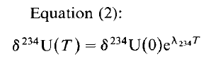
Frank et al (note to Table 1) report the use of the following equation with Th232-corrected values (and the same decay constants as Edwards 1987):

With a bit of experimenting, this proves to be equivalent to the corresponding equation in Edwards 1987 (multiplied by [U238/U234]_act ).

The Th adjustment deducts an allowance for non-U238-sourced Th-230 using the following equation (Appendix):

This adjustment requires two empirical constants: is the Th230/Th232 activity of present-day spring water (1.85 -see page 42), used here as an approximation for ancient spring water, while is the Th230/Th232 activity of detritus estimated at 0.526 (based on a sample from a nearby travertine site (Hass/Lauster).

I’ve tried pretty hard to replicate the results in Frank et al 2000 and have got close, but can’t quite replicate them. Without being able to do so, it’s impossible to test the Th-adjustments in Fleitmann et al 2007. For what it’s worth, here is my attempt to replicate the calculations of Frank et al 2000:

First, here are the constants collated from various locations in the paper:

lambda=NULL; lambda[“Th230”]= 9.195E-6#Table 1 Frank
lambda[“U234”]= 2.835E-6 # Table 1
lambda[“U238”]= 1.551E-10 #Table1
R0=1.85;Rd=.526

Next here is the information in Frank Table 1, collated by cut and pasting from the pdf into Notepad and tidying:

A=read.table(“http://data.climateaudit.org/data/speleothem/Frank.2000.edited.dat”,sep=”\t”,header=TRUE)

Next here is an implementation of the function in Frank et al 2000, combining the equation in the note to Table 1 (the one that corresponds to Edwards 1987 Equation 1) and the Th-adjustment equation in the Appendix.

f=function(t) {
X=act.Th230_U234-act.Th232*(R0-Rd)*exp(-lambda[“Th230”]*t)-act.Th232*Rd #equation A1
B=act.U238_U234* (1-exp(-lambda[“Th230”]*t) )
C= (1- act.U238_U234)* lambda[“Th230”]/(lambda[“Th230”]-lambda[“U234”])
D= (1- exp( -(lambda[“Th230”]-lambda[“U234”])*t) )
f= (X- (B+ C*D) )^2
f}

Now I solved the non-linear equation for each set of measurements, setting non-converging to NA:

K=nrow(A); age=rep(NA,K)
for(i in 1:K) {
act.Th230_U234=A$act.Th230_U234[i]
act.U238_U234=1/A$act.U234_U238[i];
act.Th232=A$act.Th230[i]/A$act.Th230_Th232[i]
age[i]= optimize(f,interval=c(0,200000),tol=1E-6)$minimum
}
names(age)=A$sample
age[(abs(age-200000)<1)]=NA

Next I collected the results and reported the comparison to the corresponding results in Frank Table 1:

test=data.frame(names(age),A$height_m,round(age,0),A$age*1000,round(age- A$age*1000,0) )
dimnames(test)[[2]]=c(“Sample”,”Height_m”,”Repl(corr)”,”Frank”,”Diff”)
test

This yielded the following results, with the results being sort of close, but nothing quite matched. The differences were all within the “error” shown in the Table, but that seems to me to be a different sort of issue – the numerical results should match exactly.

Right now, I don’t have any idea why my results don’t quite match. So it becomes hard to proceed to analyze Fleitmann et al 2007 without being able to benchmark the dating procedures. Perhaps I’ve misplaced a sign somewhere or made some other slip. The replication is pretty good, which makes it that much harder to sort out what, if anything, I’ve done wrong. As I’ve shown here, the age calculations take only a few lines – if you don’t believe me, run the scripts. Frank et al 2000 documented their lab procedures very carefully; wouldn’t it be nice if they did the same for their statistical procedures.