Here’s a pretty little graph that I think that you’re going to see more of. One is using the Wahl-Ammann variation of MBH methodology applied to MBH data; the others are from low-order red noise. 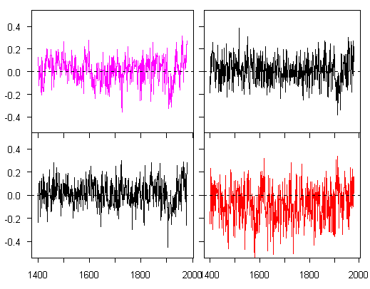
Pink – no PC reconstruction from WA without strip-bark and Gaspé; black – from low-order red noise.
I worked this up to illustrate a point in the no-PC part of Wahl and Ammann, but it bears a little commentary separately. You may recall jae trying to wrap his mind around overfitting and bender getting frustrated with him. If it makes either of them happier, MBH – WA variation – is a wonderful example of overfitting that may illustrate the point for jae, who might then undertake to explain the problems to Ammann and Wahl.
The pink graphic is the no PC reconstruction from WA without strip-bark and Gaspé, resulting in a network of 70+ series (down from the 95 in their Scenario 2 due to the strip-bark sites.) If you did a multiple linear regression of NH temperature against 70+ series with little mutual relationsip in a calibration period of length 79, I think that you’d agree that it was overfitting. So what would a reconstruction look like from such a process? I haven’t illustrated that here (I’ll do that now that I think of it), but it would look a lot like the above graphic.
Here I’ve used PLS (partial least squares) rather than OLS- see my linear algebra posts as to the proof that MBH regression can be reduced to partial least squares. OLS multiplies the partial least squares coefficients by  . If the network is close to orthogonal, then the PLS coefficients will not be changed all that much. In the simulations, to do it quickly, I’ve used a simple network with AR1=0.2 and then re-scaled the variance to match that of the series being illustrated. As you can see, there’s negligible visual difference between the MBH result and red noise.
All the reconstructions have high r2 (greater than 0.5) in the calibration period, and ~0 verification r2. This would be enough for non-climate scientists to conclude that there was overfitting.
Another distinctive feature of overfitting is the characteristic downward notch at the start of the calibration period – this is worth paying close attention to in the WA diagrams where it’s all too visible.
In the red noise and non-bristlecone cases, the reconstruction reverts to close to zero fairly quickly. If you re-insert bristlecones or HS-shaped series, their impact is to change the shaft location to more and more negative, while preserving the general geometry. I’ve been alking about the interrelation of spurious regression and overfitting for some time without illustrating it as clearly as I’d like. Fortunately, the Wahl and Ammann variation has introduced overfitting on such a colossal scale that it’s easy to show the effect.
I doubt that anyone in our lifetimes will ever again see elementary overfitting on the scale of Wahl and Ammann.