New Nic Lewis Paper

Nic Lewis’s paper on climate sensitivity is available. See his BH post here. Also see discussion at Judy Curry and WUWT.

Tingley and Huybers Exclude Mt Logan

Perhaps the greatest single difference between being a “real climate scientist” and policies recommended here is that “real climate scientists” do not hesitate in excluding data ex post because it goes the “wrong” way, a practice that is unequivocally condemned at Climate Audit and other critical blogs which take the position that criteria have to be established ex ante: if you believe that treeline spruce ring widths or Arctic d18O ice core data is a climate proxy, then you can’t exclude (or downweight) data because it goes the “wrong” way.

This seems trivially obvious to anyone approaching this field for the first time and has been frequently commented on at critical blogs. However it is a real blind spot for real climate scientists and Tingley and Huybers are no exception.

Fisher’s Mount Logan ice core d18O series is a longstanding litmus test. It goes down in the latter part of the data and is not popular among multiproxy jockeys. Tingley and Huybers excluded Mt Logan from their data set, purporting to justify its exclusion as follows:

We exclude the Mount Logan series that is included in [35] because the original reference [36] indicates it is a proxy for precipitation source region and is out of phase with paleotemperature series.

In the figure below, I show two Arctic d18O series – on the top is Windy Dome, a Thompson series from Franz Josef Land used by Tingley and Huybers and on the bottom is the Mt Logan series that they excluded.

two ice core proxies
Top: d18O. top- Windy Dome, Franz Josef. bottom – Mt Logan.

Windy Dome d18O goes up in the 19th and 20th century. The possibility that some portion of the increase might be attributable to change in source region doesn’t cross Tingley and Huybers’ mind. On the other hand, Mt Logan goes down and the authors unhesitatingly attribute this to change in source precipitation and exclude it from their network (post hoc.)

However, they don’t consider the bias inherent in this sort of ex post exclusion. Attributing the decrease at Mt Logan to changes in precipitation source is very plausible. But it’s equally plausible and even probable that changes in precipitation sources could also work in the opposite direction, exacerbating any increase due to temperature. Perhaps there was a change in source region for Windy Dome that contributed to its recent increase in d18O values. Exclusion of Mt Logan, without a compensating exclusion of an accentuated upward series, will impart a bias to any composite.

If scientists believe that Arctic d18O is a proxy for temperature, then they cannot exclude data after the fact because it goes the “wrong” way, as Tingley and Huybers have done here. Particularly if they have no compunction about using contaminated data that goes the “right” way.

If authors take longer to report data that goes the “wrong way”, this will also bias composites at any given time. For example, Lonnie Thompson’s Bona-Churchill series, which is near Mt Logan, also goes the wrong way. Has this contributed to the delay (now exceeding 10 years) in reporting these results?

Tingley and Huybers: Varve Compaction

Specialist literature on varves e.g. Besonen et al 2008 – coauthor Raymond Bradley -(which is cited by Tingley and Huybers) make the obvious observation that varves are compacted within a core. Besonen et al 2008 allow for compaction by estimating annual mass accumulation as a more appropriate measurement of varve “thickness”, rather than uncompacted varve thickness. In their abstract, Besonen et al stated:

In many studies of lakes from the High Arctic, varve thickness is a good proxy for summer temperature and we interpret the Lower Murray Lake varves in this way. OnOn that basis, the Lower Murray Lake varve thickness record suggests that summer temperatures in recent decades were among the warmest of the last millennium, comparable with conditions that last occurred in the early twelfth and late thirteenth centuries, but estimates based on the sediment accumulation rate do not show such a recent increase

They report later in the article:

On the other hand, because of compaction, the thickness of recent varves is not directly comparable with those varves that are buried deeper in the sediment pile. This problem can be addressed by calculating a packing index (a simple ratio of the area occupied by sediment grains versus the area occupied by matrix in the varve BSE images) and then calculating the sediment accumulation rate on an annual basis (assuming a constant sediment density of 2.65 g/cm3, for quartz). This procedure compensates for compression of the sediment with depth, and results in a suppression of the trend over the last century seen in the varve thickness record (Figure 7).

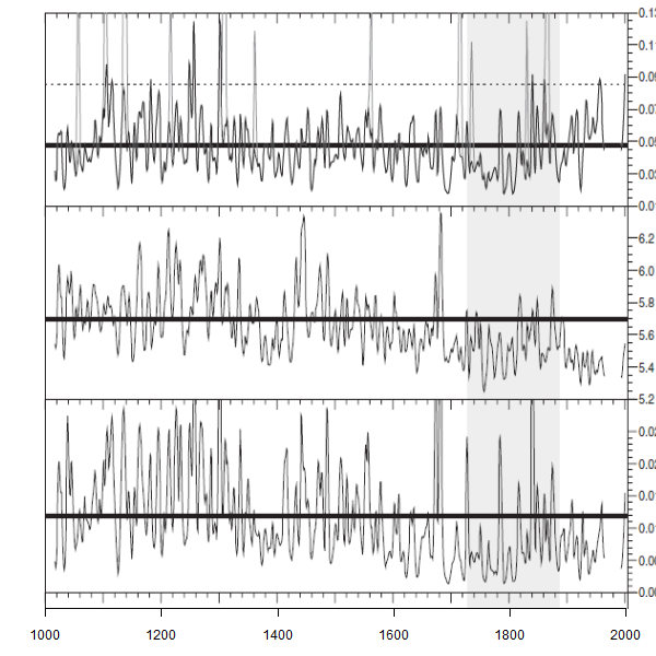
An excerpt from Besonen’s Figure 7 is shown below. The top panel shows varve thickness unadjusted for compaction, while the bottom panel shows mass accumulation. The top panel (with no allowance for compaction) shows somewhat elevated 20th century levels, while the bottom panel (after allowing for compaction) does not – the phenomenon noted in their abstract.

besonen excerpt
Figure 1. Excerpt from Besonen et al Figure 7. Top – varve thickness unadjusted for compaction (but after turbidites); middle – density; bottom – mass accumulation.

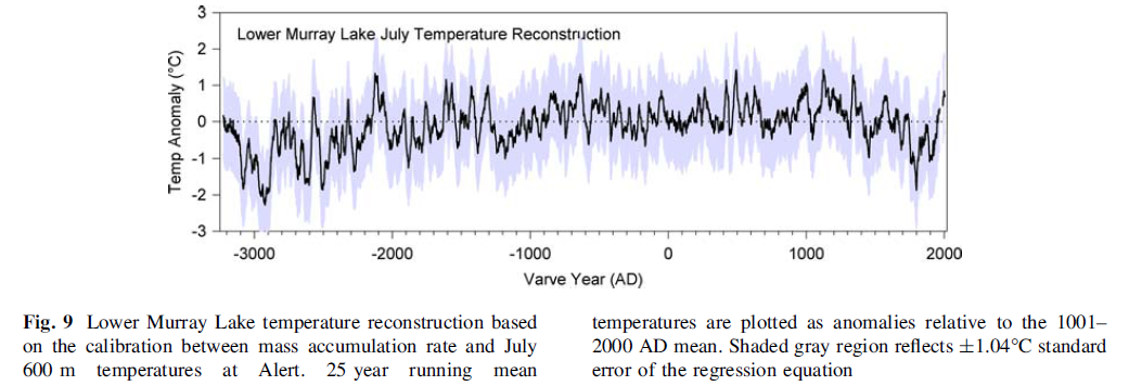
A related article (Cook et al 2009 – also with Bradley as coauthor) the following year on a different Murray lake core made similar observations about compaction. Cook et al provided a temperature reconstruction using mass accumulation rate, showing a rather elevated MWP as shown below. I’m not inclined to put much weight on simplistic reconstructions from varve thickness (see also my discussion of Gifford Miller’s observations on this topic), but show this series as evidence that mass accumulation was used by this group as the relevant index.)

cook excerpt re murray lake
Figure 2. Excerpt from Cook et al 2009.

Tingley and Huybers 2013 have three classes of proxy data: MXD data, which has the familiar divergence problem; ice core O18 which doesn’t have a Hockey Stick shape and varves. The Murray Lake varve series is used. Tingley and Huybers provide an excellent SI, including exact URLs for data sets as used – a simple enough protocol that unfortunately is seldom observed. (They forgot to archive their actual reconstruction, though I presume that this is a mere oversight since their intent is clearly to provide a comprehensive archive).

In their SI, they state:

Details and references for the lake varve records used in the analysis are available in Table S.1. Unless the description of the data indicates otherwise, we use the total varve thickness.

Of the two Murray Lake versions (different cores taken by the same group), they cite the Besonen et al version.

For the Murray lake record, we use the unfiltered version of the shorter (1000 year) record posted at the NOAA Paleolimnology site [60].

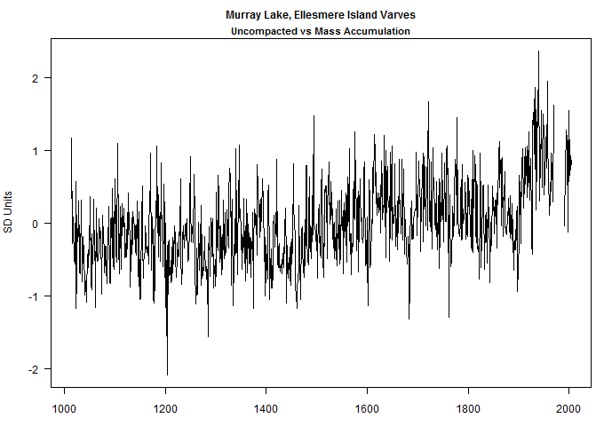
However, when one compares their archive of data as used to the NOAA archive, one can immediately determine that they used varve thickness without compensating for varve compaction (the series match), rather than mass accumulation as used by Cook et al 2009 in their temperature reconstruction. This decision gives a pronounced upward bias, as shown by the difference between the two series (after taking a log and then scaling as in Tingley and Huybers.)

Murray uncompacted difference
Figure ^. Murray Lake. Difference between uncompacted varve thickness as used by Tingley and Huybers and mass accumulation. Both series logged and then scaled, before differencing.

I haven’t yet looked at how the other varve series handled compaction, but it seems like an important issue in any attempt to deduce temperatures from this sort of data. In the particular case of the Murray Lake series, it seems to me that the original data clearly “indicates” that mass accumulation be used as an index, rather than varve thickness unadjusted for compaction and that this should have been used according to the stated methodology of Tingley and Huybers.

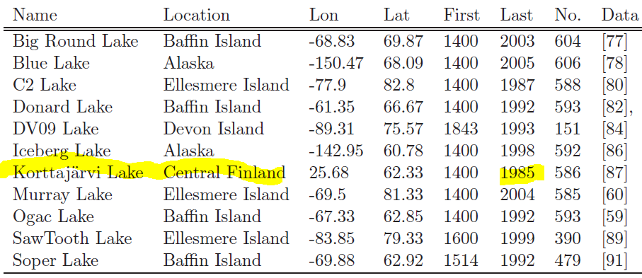
As previously noted, Tingley and Huybers also used the contaminated portion of the Korttajarvi sediment data, so there are multiple problems with their varve reconstruction. These are not complicated issues, but ones that ought to be within the scope of even Nature peer reviewers.

New Light on Svalbard

In 1997, the 121 m Lomonosovfonna ice core was drilled in Svalbard. As of mid-2009, when Hu McCulloch and I wrote CA posts on this core, nothing had been published on
O18 values prior to AD1400 nor had any Lomonosovfonna data been archived, even for the post-1400 period.

Both Hu McCulloch and I, in separate CA posts here and here, speculated that the withheld O18 values prior to AD1400 would elevated values. A digital version of the pre-1400 data became available this week in connection with Hanhijarvi et al and confirmed our surmise, as shown below. Continue reading

More from the Junior Birdmen

A new paper in Nature by Tingley and Huybers h/t WUWT.

In keeping with the total and complete stubbornness of the paleoclimate community, they use the most famous series of Mann et al 2008: the contaminated Korttajarvi sediments, the problems with which are well known in skeptic blogs and which were reported in a comment at PNAS by Ross and I at the time. The original author, Mia Tiljander, warned against use of the modern portion of this data, as the sediments had been contaminated by modern bridgebuilding and farming. Although the defects of this series as a proxy are well known to readers of “skeptical” blogs, peer reviewers at Nature were obviously untroubled by the inclusion of this proxy in a temperature reconstruction.

tingley table s1

They stated:

For the Korttajarvi Lake record, we use the organic layer thickness, as the original publication indicates that a thicker organic layer “probably indicates a warmer summer and a relatively long growing season” [57- Boreas].

However, they didn’t mention the following:

This recent increase in thickness is due to the clay-rich varves caused by intensive cultivation in the late 20th century.

and again:

In the 20th century the Lake Korttaja¨rvi record was strongly affected by human activities. The average varve thickness is 1.2 mm from AD 1900 to 1929, 1.9 mm from AD 1930 to 1962 and 3.5 mm from AD 1963 to 1985. There are two exceptionally thick clay-silt layers caused by man. The thick layer of AD 1930 resulted from peat ditching and forest clearance (information from a local farmer in 1999) and the thick layer of AD 1967 originated due to the rebuilding of the bridge in the vicinity of the lake’s southern corner (information from the Finnish Road Administration). Varves since AD 1963 towards the present time thicken because of the higher water content in the top of the sediment column. However, the gradually increasing varve thickness during the whole 20th century probably originates from the accelerating agricultural use of the area around the lake.

All of this was discussed ad nauseam following Mann et al 2008, though Mann stubbornly refused to concede anything. Kaufman et al 2009 also used the data and, on the advice of Overpeck, conceded the point and issued a corrigendum. Raymond Bradley was a coauthor of both papers and more or less simultaneously took the position that a corrigendum was required and not required.

I’m sure that we’ll be told that their use of contaminated Korttajarvi data doesn’t “matter” – nothing ever seems to. But why use it?

Steve Update Apr 11:
For R users, I’ve collated the Tingley proxies into a time series R-matrix called proxy.tab at http://www.climateaudit.info/data/multiproxy/tingley_2013 and their metadata as info_tingley.csv. A simple average of all the Tingley proxies is shown below. It has a divergence problem because the majority of proxies are MXD proxies.

tingley_avg

Their Figure S34 top panel shows a reconstruction from MXD proxies along. The reconstruction is very similar to an MXD average,as shown below.
mxd-recon
Figure ^. Tingley and Huybers S34 top panel, showing one variation of their proxy-only reconstructions (MXD), with average of MXD proxies (green) for comparison.

Tingley has provided an exemplary archive. It requires a little collation. R users who wish to skip their own collation may use my collation as follows:

download.file("http://www.climateaudit.info/data/multiproxy/tingley_2013/proxy.tab","d:/temp/temp",mode="wb")
load("d:/temp/temp")
tsp(proxy) #1400 2005

info=read.csv("http://www.climateaudit.info/data/multiproxy/tingley_2013/info_tingley.csv")
dim(info)	#[1] 125  11

annual=ts(apply(scale(proxy),1,mean,na.rm=T),start=1400)
count=ts(apply(!is.na(proxy),1,sum),start=1400)
max(time(count)[count>20]) #1992

#png(file="d:/climate/images/multiproxy/tingley_avg.png",w=680,h=480)
plot.ts( window(annual, end=max(time(count)[count>20]) ),ylab="SD Units")
title("Average of Normalized Tingley Proxies")
abline(h=0,lty=3)
#dev.off()

The Impact of TN05-17

TN05-17 is by far the most influential Southern Hemisphere core in Marcott et al 2013- it’s Marcott’s YAD061, so to speak. Its influence is much enhanced by the interaction of short-segment centering in the mid-Holocene and non-robustness in the modern period. Marcott’s SHX reconstruction becomes worthless well before the 20th century, a point that they have not yet admitted, let alone volunteered.

Marcott’s TN05-17 series is a bit of an odd duck within his dataset. It is the only ocean core in which the temperature is estimated by Modern Analogue Technique on diatoms; only one other ocean core uses Modern Antalogue Technique (MD79-257). The significance of this core was spotted early on by ^.

TN05-17 is plotted below. Rather unusually among Holocene proxies, its mid-Holocene values are very cold. Centering on 4500-5500 BP in Marcott style results in this proxy having very high anomalies in the modern period: closing at a Yamalian apparent anomaly of over 4 deg C.

TN05-17_baseFigure 1. TN05-17.

In the most recent portion of the Marcott SHX, there are 5 or fewer series, as compared to 12 in the mid-Holocene. Had the data been centered on the most recent millennium and extended back (e.g. Hansen’s reference station method is a lowbrow method), then there would have been an extreme negative contribution from TN05-17 in the mid-Holocene, but its contribution to the average would have been less (divided by 12, instead of 4). As shown below, TN05-17 pretty much by itself contributes the positive recent values of the SHX reconstruction. It’s closing anomaly (basis 4500-5500 BP) is 4.01 deg. There are 4 contributing series – so the contribution of TN05-17 to the SHX composite in 1940 is 4.01/4, more than the actual SHX value. The entire increase in the Marcott SHX from at least 1800AD on arises from increased influence of TN05-17 – the phenomenon pointed out in my post on upticks.
TN05-17 contribution
Figure 2. Contribution of TN05-17 to the Marcott SHX reconstruction.

Given the overwhelming importance of this proxy, one would like to know a little more about it. The next graphic compares TN05-17 to two other SHX proxies, also MAT proxies but from small lakes in southern New Zealand. The inconsistency of the proxies is evident. The New Zealand paleolimnological proxies have nothing resembling the mid-Holocene “cold period” that characterizes TN05-17. One thing that this graphic shows for sure: the residuals of these proxies from the “true” temperature history as translated to the respective sites do not remotely resemble a low-order AR1 process. To properly model the error distribution, one has to have an error model that permits excursions for millennia – not at all easy to specify.

SHX MAT proxies
Figure 3. Three SHX Modern Analogue Technique Proxies

It appears highly probable that there is some confounding influence on TN05-17. TN05-17 was cored in the Atlantic sector of the Southern Ocean south of Africa. As shown in the graphic below, it is located in very large scale “sediment drifts”.

agulhas drift annotated
Figure 4. Location map of TN05-17 (shown as red dot.)

Nielsen et al 2004 observed that the alkenone temperatures of the most recent samples are several degrees higher than ocean temperatures in the area. They speculated that some of the coretop might be missing – not particularly reassuring when this proxy is the most important contributor not just to 20th century SHX Marcott warming but 19th century SHX Marcott warming. There is occasional discussion in specialist literature of circumstances in which alkenone temperatures are warmer than local ocean temperatures e.g. Ruhlemann et al taking the alkenones from the warmer location in which they formed to the colder place where they settled:

We suggest that the southern samples are biased by suspended organic detritus originating from the cold subpolar waters of the northward flowing Malvinas Current, whereas the northern samples carry an UK’37 signal of tropical/
subtropical origin, transported southward with the Brazil Current. On the basis of surface ocean transport pathways and velocities simulated with the large-scale geostrophic (LSG) ocean general circulation model, we identify areas of the world ocean where alkenone temperatures are potentially biased to higher or lower values due to long particle residence times and lateral advection by surface currents.

The area studied by Ruhlemann et al was in the western South Atlantic between 30 and S. Could something similar be going in the eastern South Atlantic in the area of TN05-17 (50S, 6E) – seems entirely possible to me. There is convincing evidence that there have been secular changes in the Agulhas currents over the Holocene. The TN07-17 history certainly suggests secular changes to me: it looks like ocean currents have changed in this sector over the Holocene, such that alkenone drift (along the lines of the South American alkenone drift) has contributed to the warm values in the early Holocene and later Holocene, while colder currents were present in the mid-Holocene.

Whatever is right or wrong about Marcott et al, merely from a perspective of craftsmanship, it is not particularly reassuring that the main (Yad061 even) contribution to modern SHX warming in the Marcott reconstruction appears to arise from a “cold” mid-Holocene interval at TN05-17, translated into modern warming through short-segment mid-Holocene centering and modern proxy dropout.

Alkenone Divergence offshore Iceland

The longest very high-resolution alkenone core that I’m aware of is Sicre et al’s MD99-2275 (plus splices) from offshore Iceland (67N 18W). It is 4550 years long, its most recent value is 2001AD and its resolution is 4 years. Marcott used nearby core JR51GC-35 (also at 67N 18W), also an alkenone record, which had a resolution of 110 years and a most recent Marcott date of 1836AD.

Here is how the two series compare over the 4500 years covered by the Sicre et al record (originally published in 2008, but updated in 2012). (The NOAA archive is unfortunately inadequate as it does not include depth or identify splice points.)

iceland 67N 18W modern
Figure 1. 67N 18W Offshore Iceland. Comparison of Marcott et al series to high-resolution series.

Taking a longer view, here are the two series compared over the Holocene.

MD99-2275-comparison-long
Figure 2. 67N 18W Offshore Iceland. Comparison of Marcott et al series to high-resolution series.

Finally, here’s a zoom into the modern period.
iceland 67N 18W highres
Figure 3. As above. Zoom in.

In geophysical surveying, one tries to use the best quality surveys where available and benchmark lower quality surveys against the highest quality ones. If this methodology were used here, the errors in JR51GC-35 are obviously very large, much higher than arising from the alkenone calibration equation by itself, though other factors could be at work as well.

MD99-2275 has well-dated core going deep into the Holocene. Hopefully, Sicre and other specialists will continue their commendable program. Seeing if these results can be replicated in another core would also do much to increase confidence.

The alkenone divergence problem is clearly present in this data. ALkenone-estimated temperatures in the 20th century continued to decline. In the Marcott reconstruction, JR51GC-35 makes its last (very negative) contribution in the 1820 step. By the act of no longer participating, it causes the Marcott composite to go up in the next period, even though it appears that the “true” alkenone estimated temperature in the area continues to decline.

Postscript:
I mentioned MD99-2275 as a high-resolution core in my notes on AGU 2006. Like McGregor’s Cape Ghir (used inverted), it was one of the proxies in Trouet et al 2009 discussed at CA here. Here is a figure showing the updated Sicre version against the Trouet et al illustration. The Sicre version is in cyan (versus the “Iceland” series in blue). The divergence in the present series continues further than in the Trouet version.

trouet-2009-annotated
Figure 4. Excerpt from Trouet et al 2009, showing updated Sicre et al series.

Alkenone Divergence in Peru

Gutierrez et al (GRL 2011) pdf here; data here is another very high resolution alkenone series that is well-dated in the 20th century. It was taken in an upwelling zone offshore Peru at a similar latitude to Quelccaya.

Like the high-resolution series offshore Morocco and Namibia, it shows a sharp decline in alkenone-estimated SST in the 20th century, as illustated below. (The archived data has a little more coverage -back to ~1750.)

B0406 alkenone
Excerpt from Gutierrez at al 2011.

The authors survey temperature data at nearby stations (Callao, Pisco and a few others) and report slight cooling in the late 20th century. They suggest “ERA 40 reanalysis indicates its link [cooling] with intensified alongshore winds driving upwelling in spring”.

The closest Marcott proxy is GeoB7139-2, taken offshore Chile at approximately 30S. (A closer comparison would be nice.) This proxy is shown below. It only has two radiocarbon dates in the entire Holocene and only has resolution of ~520 years. (Stated data selection criteria are that “at least four age-control points span or closely bracket the full measured interval” and “sampling resolution is typically better than ~300 yr”.

GeoB7139-2
Figure 2. GeoB 7139-2 per Marcott.

The next graphic shows GeoB7139-2 together with B0604 (the latter offset by 4 deg C).
B06045 comparison
Figure 3. B0604 (offset 4 deg C) and GeoB7139-2.

Although we’ve been reassured by Marcott apologists of the ability of their data and method to capture any past upspike, one feels that this particular series will not be much help in that enterprise.

In Lonnie Thompson’s recent Quelccaya publication, Thompson estimated Nino3-4 SST. Needless to say, they don’t bear much similarity to the alkenone SSTs shown here.

Stepping back from Marcott, increased upwelling in the late 20th century seems to have occurred all over the globe. In addition to the upwelling sites surveyed here in the last couple of days (Morocco, Namibia, Peru), I’ve also seen 20th century declines in alkenone data offshore Iceland and, of course, in the two Marcott series where the decline was deleted: MD03-2421 offshore Japan and OCE326-GGC offshore eastern Canada, both of which I’ll now reconsider with this in mind.

Alkenone Divergence

While there are disappointingly few high-resolution alkenone ocean cores with 20th century resolution, there are a few. Given the importance of this class of proxy in Marcott et al, one would have thought the performance of high-resolution alkenones in the 20th century would have been of interest to Marcott et al, but they were silent on the topic.

Before Climategate, I’d considered high-resolution ocean cores from time to time at Climate Audit (see alkenone tag). In 2007, I reported on a very high-resolution alkenone series offshore Morocco (about 30N) by Helen McGregor (see here and here). This dataset had a serious divergence problem, i.e. the water was getting colder. McGregor worried that fish in the area might need swimming lessons to cope with the rapid change.

McGregor’s series was cited in Leduc et al (2010), a specialist presentation of another high-resolution alkenone series (GeoB8331, GeoB 8331) taken in the Benguela upwelling zone offshore Nambia at about 30S. Like McGregor, they also found sharply cooler SST in late 20th century as measured by well dated alkenone data, indicating that the alkenone divergence problem was not unique to McGregor’s site:
leduc benguela sst
Figure 1. From Leduc et al 2010.

The closest Marcott series to McGregor’s Morocco series was the Iberian Margin (#51) D13822 alkenone series (Abrantes et al.) The graphic below compares the two series: the shorter (warmer) high-resolution McGregor series in red and the longer series used by Marcott in black. The green “rug” marks at top are D13822 radiocarbon dates.

iberian-margin-long

The next graphic shows the modern portion of these two series, both offset to facilitate comparison. In this graphic, I’ve both the published and Marcott dates for the Iberian Margin series, together with the high-resolution McGregor series. All show very pronounced closing downticks, with the well-dated McGregor series placing the Morocco decline in the 20th century and even the last half of the 20th century, Marcott dating the decline in the Iberian Margin to the 19th century (with a dating error of 100-150 years) and Rodrigues et al dating the decline to the 15th century. An obvious question is whether the downturns in the Iberian Margin and Morocco series are contemporary or phased. (Note that the removal of D13822 after the late 19th century contributed to the Marcott 20th century uptick.)

iberian-margin-modern

Both sites are very high accumulation. McGregor’s box core GeoB6008-1 accumulated 32 cm in less than a century (1912-1998), while the Iberian margin D13822 is estimated to have accumulated about 25 cm per century (this is about 20 times higher than many cores.) The top sample for D13822 is at 10 cm and dated 57BP by Marcott and 442 BP in the original publication (which I haven’t seen yet.) The closest radiocarbon date is at 257 cm (calibrated 1511 BP) i.e. not closely dated. For comparison, the 10 cm sample in closely-dated GeoB6008-1 is dated to 1981AD and to 1947AD in GeoB6008-2.

Trouet et al 2009

As an amusing sidebar, we also discussed the McGregor alkenone series as it was used in a multiproxy study by Trouet et al 2009 – see CA discussion here. Trouet “solved” the divergence problem in best Mann et al 2008 style: by turning the series upside down. The red series labelled “Cape Ghir” and going sharply upward in the excerpt from Trouet et al 2009 is the McGregor alkenone series with sharply colder temperatures.


Excerpt from Trouet et al 2009.

The practice of multiproxy authors turning indicators of cold SST upside down had been previously criticized at CA in connection with Moberg et al 2005, which used a proxy series showing increased presence of coldwater (polar) foraminifera (% G Bulloides) in the Arabian Sea as one of their most potent indicators of global warming.

The closest Marcott series to the Leduc et al 2010 Benguela series shown above is Farmer’s ODP1084B (also used in Loehle and McCulloch and discussed in Schmidt’s critique of Loehle and McCulloch.) I’ll discuss this interesting downspike on another occasions.

In general, 20th century downspikes in high-resolution alkenone series seem to be the rule, rather than the exception – a divergence problem that is not discussed in the multiproxy studies. The most plausible reason is that high-resolution in the 20th century requires high-resolution, which requires high biological productivity, which, in turn, is most characteristic of upwelling zones. Increased upwelling in upwelling zones seems to be a rather pronounced in the 20th century. This is not inconsistent with overall warming, but neither is it an issue that multiproxy jockeys can simply brush aside.

Clearly distinguished

[Update 04/08/13: Josh has once again a brilliant view what’s going on here and in some other cases. Enjoy!

BirdMann_scr]

No researchers in this field have ever, to our knowledge, “grafted the thermometer record onto” any reconstruction. It is somewhat disappointing to find this specious claim (which we usually find originating from industry-funded climate disinformation websites) appearing in this forum. Most proxy reconstructions end somewhere around 1980, for the reasons discussed above. Often, as in the comparisons we show on this site, the instrumental record (which extends to present) is shown along with the reconstructions, and clearly distinguished from them.

Michael E. Mann

grafted