Some of the CA posts that I’ve found most interesting to write have been about identifying Chladni patterns in supposedly “significant” reconstructions when principal component methods have been applied to spatially autocorrelated red noise. (This is by no means a new observation, as warnings about the risks of building “castles in the air” using principal components is prominent in the older climate literature (from the 1970s), but seemingly forgotten in the IPCC period. I did several posts on Chladni patterns in the Stahle/SWM network used in MBH99 and about Chladni patterns in the Steig et al 2009 Antarctic network (in the latter case, observing that eigenvectors said in the Nature article to have physical significance were, in fact, nothing more than the expected Chladni patterns from spatially autocorrelated data in a region shaped like Antarctica.
The second half of the McShane Wyner paper applies a sort-of MBH99 style analysis to the Mann 2008 network. In their case, instead of applying PCA to the North American tree ring (and similar networks) and combining the PCs with individual proxies as in MBH, they applied principal components to the entire proxy network. Although principal components were integral to MBH99 (and to the reprise of MBH in Rutherford et al 2005), principal components are not an important feature of the majority of AR4 studies – which, for the most part, reverted back to the simple CPS methods of Bradley and Jones 1993 and Jones et al 1998 or poorly-understood RegEM.
In my earlier discussions of Mannian networks, we observed the concentration of proxies in the bristlecone area, but since then have developed some tools for analysing spatial autocorrelation that I didn’t have at the time of the original study.
Applying these methods to the Mann et al 2008 network (McShane Wyner 93 proxy selection) yields some provocative results. (Results for the Gavin Schmidt 55 proxy subset are probably similar and I’ll get to them on another occasion.)
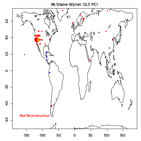
I’ve done three plots below showing weights in the style that I’ve been using – the area of the filled circle proportional to the weight. Red for positive weights, blue for negative weights. (I’ve plotted the gridcell beside Sheep Mountain in orange to avoid it being overprinted by the Sheep Mountain gridcell – there’s no significance to the orange otherwise.) In each case, I’ve added up weights in a gridcell and plotted values by gridcell. Click on the plot below for a larger version.
The figure at left show simple counts. In the Mann2008/MW93 subset, there are 24 bristlecone series, which are reflected in relatively high weights in the bristlecone area. The middle plot is the eigenvector corresponding to a PC1 from spatially autocorrelated red noise located at the locations of the actual proxies – for this calculation, I used spatiall decorrelation of exp (- distance_km/1200), a decorrelation factor more or less equivalent to what we’ve seen in station data. It’s worth experimenting with this. By working directly on the correlation matrix, you can get the eigenvector directly (you could do lots of simulations, but you don’t need to.) Notice what taking the principal component does: it focuses the weights on the bristlecone area, and makes “peripheral” weights almost negligible. This is a more extreme version of what we saw with the Antarctic Chladni patterns. There the PC1 tended to overweight the center of the region and underweight the boundary (this is the Chladni pattern of a drum). It’s even more extreme here – the Chladni pattern is really focused on the bristlecone area with negligible weights on the periphery. Take a look at the graph and I’ll discuss the actual proxy network eigenvector afterwards.

Left- Counts; middle – eigenvector for spatially autocorrelated PC1 given proxy locations; right- eigenvector for M08-MW93 network PC1.
The eigenvector for the actual proxy PC1 is “remarkably similar” (TM – climate science) to the eigenvector for spatially autocorrelated red noise at locations of the actual proxies. However, there are a few very interesting details. There are two negatively-oriented proxies in the actual PC1 in central America. The Yucatan proxy in question has a very elevated medieval warm period. Because this is antithetical to the bristlecone pattern, it is flipped over in the PC1. This is related to the phenomenon observed in McMc 2005 (EE) where we observed that proxies with a warm early 15th century introduced into an augmented network would be flipped over because of the way that bristlecones imprinted the PC1.
Other noticeable details: the two Tiljander proxies retained in the Mann 2008 (MW93) network fight the tendency to downweight “peripheral” proxies in the PC1 and are noticeably weighted. The “Tornetrask” series also receives a higher weight than in the spatially autocorrelated version – as I noted on another occasion, Briffa’s Yamal series is averaged with Tornetrask (and Taimyr) and used as “Tornetrask”.
Next, here is an interesting comparison of the eigenvalues for spatially autocorrelated red noise at actual proxy locations and for the actual M08 (MW93) proxy network. On the left is a “scree” plot showing the squared eigenvalues (log scale) for the actual proxy network as compared to spatially autocorrelated red noise. Gavin Schmidt has an eigenvalue comparison in the Schmidt et al comment on Mc_W, but does not consider the potential impact of non-random spatial distribution of proxy locations. On the right is the cumulative eigenvalue weights.
The 2nd and higher eigenvalues for the proxy network are higher than the corresponding eigenvalues for spatially autocorrelated red noise. However, the first eigenvalue for spatially autocorrelated red noise is a LOT higher than the actual network and the cumulative eigenvalue weights for the actual network are lower at all points than spatially autocorrelated red noise.
I’m mulling over the interpretation of these results, but my first impression is that the results of the actual network are forced by the unique properties of the bristlecones. The bristlecone pattern is very distinct and imprints the PC1 of the actual network; lower eigenvectors are various contrasts with the bristlecones and are more heavily weighted because the bristlecones are somewhat sui generis.

Chladni patterns are pretty interesting in themselves. In the present case, the bristlecones result in a mathematically interesting sort of symmetry-breaking.
As observed on other occasions, the NAS panel said that strip bark should be “avoided” in temperature reconstructions, but, like the dead parrot in Monty Python, they were re-sold in Mann et al 2008 (notwithstanding its claims that it complied with NAS recommendations) and included in the MW analysis. In the Schmidt comment, he says that these have been vindicated by Hughes and Funkhouser 2009 (not available at the time of Mann et al 2008), with Gavin Schmidt pointedly avoiding any discussion of Linah Ababneh’s failure to replicate Graybill’s Sheep Mountain chronology.