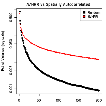
Many CA readers know a lot about regression and quite a bit about principal components, but I dare say that a much fewer number are familiar with Truncated Total Least Squares (to which the regpar parameter belongs.) We’re seeing interesting interactions between PC=k and regpar=r – and there is little, if anything, in regular statistical literature about this particular interaction in the context of spatially autocorrelated time series. Steig doesn’t cite anything.
Layered onto this methodology is an expectation-maximization algorithm, whose properties are also poorly understood. In our situation, the layering of the RegEM algorithm has the extreme disadvantage of making the underlying linear algebra even more murky. To make matters worse, the RegEM algorithm performs two very different functions: 1) it infills missing values in the station history data (which goes back to 1957); and 2) there is no satellite data prior to 1982 and it extrapolates values before 1982 – a process that is very different conceptually from simple “infilling”.
My underlying perspective on all these problems is that they are a variety of multivariate calibration and that, in order to reduce the algorithms to something remotely resembling a method known off the Island, it is necessary to connect the methods somehow to things described in Brown and Sundberg, which we’ve discussed before. In a Brown and Sundberg (1989) context, I think that RegEM, under any of its guises, can be viewed as “updating” calibration coefficients, a topic that I’ll return to.
For now, I thought that it would be useful to consider a situation where we have both PCs and Truncated Total Least Squares without RegEM and see what it does. As an experiment along these lines, I created a block-matrix structure that was “complete” except for the reconstruction – illustrated below. Let’s assume that we have a complete subset of station data over both the calibration and reconstruction period. In my example analyzed here, I’ve made a “complete” subset by only using stations with at least 240 values (out of 600) and infilling the missing values using Steig RegEM (regpar=3) purely for the sake of argument. In the example here, I’ve used 3 PCs, again purely for the sake of argument.
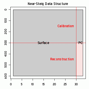
Figure 1. Steig Data Structure after PC calculation
A Calibration Perspective
The PCs are, of course, derived from the AVHRR data. In calibration terms, we calibrate the PCs versus the station data in the calibration period and use the station data in the reconstruction to derive the PCs. In calibration terms, the PCs are the X-matrix and the station data the Y-matrix. The calibration equation is as follows:
(1) 
yielding the standard OLS estimate for regression coefficients
(2) 
since the X matrix is here an orthonormal matrix of PCs.
The maximum likelihood estimate for the reconstruction (following the calibration literature) is:
(3) 
Brown and Sundberg (1987, 1989) observe that the GLS estimate is not the maximum likelihood estimate for calibration, but under many situations isn’t “too far” away from the MLE estimate. Oddly enough, the above procedure is used in MBH, though neither MBH nor the subsequent literature indicate any realization of this. A GLS estimate of the above type doesn’t have any problem with “overfitting” and this part of MBH isn’t particularly objectionable. Ironically, it’s the part that they’ve “moved on” from.
Inverse Calibration
“Regularization” arises as a problem in this literature because Mann’s RegEM switches from “classical” calibration where Y (with q columns) is calibrated against X (p columns) to an “inverse” calibration where X is calibrated against Y with q > p. The inverse calibration creates an “overfitting” problem when X is regressed against Y.
“Total Least Squares” is a form of regression. Like OLS, it yields regression coefficients. The concept is superficially attractive – unlike Ordinary Least Squares”, errors are permitted to exist in the X matrix as well as the y vector. Mechanically, TLS is solved using principal components. An augmented matrix is formed – for simplicity, let’s consider a univariate case where we have a vector X (p=1) and a matrix Y denoted as follows:
(4) 
A singular value decomposition is carried out on this augmented matrix; the TLS coefficients are derived from the eigenvector corresponding to the smallest eigenvalue. The reasoning for this is very pretty as it appeals back to the pre-matrix linear algebra definition of eigenvector.
One of the problems with moving from OLS to Total Least Squares is that people don’t know as much about it. For example, a much higher proportion of CA readers would instantly realize that regressing x against a matrix Y (with say 30-40 columns) is a recipe for problems (“overfitting”). Fewer would realize that this also applies to Total Least Squares. Fierro 1997, the TTLS reference in Steig, observes that, under many common situations, the answers from OLS and TLS are quite close. So if overfitting looks like a problem in OLS, it will be a problem in TLS and vice versa.
Truncated Total Least Squares
There are a couple of strategies for dealing with overfitting in an OLS situation.
“Truncated SVD” is a common one. Rather than inverting  , only the first k eigenvectors are used in the inversion.
Truncated Total Least Squares is pretty much the same thing – only the truncation occurs in a Total Least Squares algorithm with an augmented matrix. Fierro 1997 describes the TTLS algorithm through language that is summarized in the diagram below, shopwing the decomposition of the eigenvector matrix from SVD on the strong> augmented matrix described above. In the case illustrated here, the decomposition of the eigenvector matrix (regpar=r=3 in this case) into submatrices for the truncated TLS coefficients which are obtained through the following equation :
(5) 
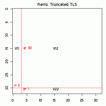
Figure 2. Diagram of TTLS Eigenmatrix Decomposition. Dimension of matrices is (n,1)= (n, q+1-r) * (q+1-r,1) * (1,1).
Total Least Squares is a special case of Truncated Total Least Squares in which regpar=q. In that case, the coefficients only involve the (q+1)th eigenvector (which has the smallest eigenvalue) and the TLS coefficients can be expressed as:
(6) 
The coefficients for Truncated TLS with regpar=1 are proportional to rows 1:q of the eigenvector corresponding to the PC1. The coefficients for TTLS (regpar=2,…, q-1) are, in a sense, intermediate between the PC1 solution and the TLS solution, yielding a one-parameter arc of line segments, analogous in a sense to the one-parameter arc between PLS and OLS solutions that we’ve observed in previous posts e.g. here – a picture that I personally find very helpful in de-mystifying these things.
Averages from USV^T Expansions
An extremely important property of the above algebra is that TTLSr (TTLS using regpar=r) yields a matrix of coefficients  . This is not a magic matrix, but merely one of many possible multivariate methods. To my knowledge, there are no commandments mandating the use of this matrix.
Because the TTLSr relationship can be reduced to a matrix of coefficients , the ultimate Antarctic temperature index (or any regional composite such as the West Antarctic average or indeed any gridcell) proves to be a linear weighting of the underlying station histories. This is something that is not understood by the Team (and in places denied), but it is easily seen from the underlying algebra – algebra which I’ve implemented in my MBH emulation, saving millions if not billions of calculations.
The demonstration below uses the “associative” property of matrix multiplication. First we denote the TTLSr estimate as follows:
(7)  .
.
where  are the reconstructed PCs (using regpar=r). In this context, they correspond to the reconstructed X-matrix in the usual X-Y matrices. In the following lines, I’ll denote here simply as
  .
.
The original PC decomposition of the AVHRR data (denoted below as  ) can be expressed in usual SVD nomenclature, taking care to observe that this SVD decomposition is distinct from the one just done on the augmented matrix, as follows:
(8) 
where  in this context is the AVHRR eigenvector (and is a different eigenvector matrix than the augmented matrix used in the calibration). Steig (as in MBH) obtains the reconstructed matrix of Antarctic gridcells
  by using the reconstructed PCs as follows:
(9) 
where  and
and  are restricted to k=3 columns.
The Antarctic average (denoted here as  is an average of the gridcells (equal area here by construction), which can be expressed as a right multiplication of the matrix as follows:
(10) 
where  here denotes a vector of 1’s of length m=5509 gridcells. Collecting the terms used to derive , we find:
(11) 
In other words,
(12) 
where  is the matrix of station data,
  is a vector of length q representing weights for each of the stations denoted in the above equation:
(13) 
Thus,
(14) 
using the definitions above for the V matrices.
This can easily be changed into a function of pc and regpar. I plotted the contribution of each station to the Antarctic average temperature, color coding the contribution by location class: green for the oddly-included islands (Campbell, Macquarie, Orcadas, Signy, Grytviken), cyan for the peninsula (9 stations out of the subset of 30 stations used here) and red for the remainder (16 stations, of which McMurdo and Scott Base are at near duplicate locations.) This yields the following barplot of weights.
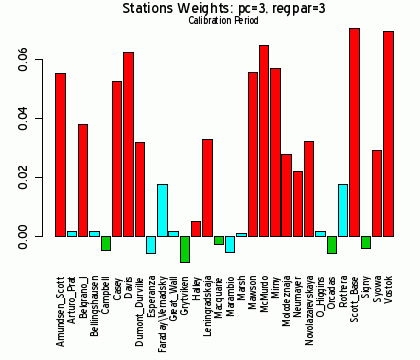
Figure 3. Effective weights in Antarctic average of 30 stations with: prior infilling of stations with more than 240 values; regpar=3, pc=3, coefficients from calibration period.
The 1957-2006 trend of this particular reconstruction is 0.061, noticeably less than the Steig trend using regpar=3, pc=3 and similar to values obtained through other methods. I’m not sure why this yields a lower trend than the RegEM’ed method. I’ve got a couple of variations in the method here : (1) the calibration coefficients from the calibration period were not “updated” from information from the reconstruction period. The interpretation of such updating is discussed in Brown and Sundberg 1989 (and isn’t easy); (2) the station data is infilled first, prior to calibration to the PC data and “short” stations weren’t used. Perhaps these lead to a difference.
IMO, it’s extremely important to keep in mind that any of these methods merely yields weights for the stations. This particular calibration ends up with relative low weights for the Peninsula stations, slightly negative weights for the Southern Ocean islands – the usefulness of which has never been clear – and relatively consistent weights for continental stations.
This sort of graph would be a helpful template for understanding what happens with varying regpar and PC. In order to end up with Steig’s trend (nearly double the trend shown here), the weights of high-trend stations have to be increased.
Trends
There’s one more potential simplification that’s useful to keep in mind. The trend of the Antarctic average can be obtained by left multiplying by a structured matrix  – see script below for definition). By expanding , we immediately see that the overall trend in
  is simply a linear weighting of the individual station trends multiplied by the vector of weights .
(15)