Santer's Boss Seeks to "Clarify Mis-Impressions"

David Bader, PhD, the Director, Program for Climate Model Diagnosis and Intercomparison, writes today seeking to “clarify several mis-impressions on your “climateaudit.org” web site” regarding the archiving of Santer’s data, the correspondence being shown below.

Readers may recall an earlier post here in which I requested data from Santer et al 2008, in response to which Santer refused to provide the data, circulating his discourteous refusal to 17 coauthors (none of whom had been copied in the original inquiry) and the journal editor. Santer:

… I see no reason why I should do your work for you, and provide you with derived quantities (zonal means, synthetic MSU temperatures, etc.) which you can easily compute yourself. I am copying this email to all co-authors of the 2008 Santer et al. IJoC paper, as well as to Professor Glenn McGregor at IJoC.

I gather that you have appointed yourself as an independent arbiter of the appropriate use of statistical tools in climate research. Rather that “auditing” our paper, you should be directing your attention to the 2007 IJoC paper published by David Douglass et al., which contains an egregious statistical error. Please do not communicate with me in the future.

I have reviewed this post and fail to see any statements by me that could possibly be construed as contributing to a “mis-impression”. On Nov 24, I reported on my unsuccessful FOI request to NOAA for the data, in which all of the NOAA coauthors claimed to have never seen the requested data. Again, I am unable to see any statements by me that could be construed as creating a “mis-impression”. The facts are what they are.

On Dec 28, I reported on efforts to obtain the data through the journal, reporting that these efforts had also been unsuccessful, as the publisher of the journal, the Royal Meteorological Society lacked a data archiving policy. A positive outcome of this effort was that the Society plans to review their lack of policy at a forthcoming editorial meeting. Again, I am unable to see any statements by me that could be construed as creating a “mis-impression”. The facts are what they are.

Around January 18th, I received a snail mail letter from the U.S. government dated Dec 10 (snail mail indeed), advising me that the FOI request had been placed in a queue and would be responded to when it got to the top of the pile. I didn’t plan to hold my breath.

On Jan 26, Ross and I submitted an article on Santer et al 2008, noted up the next day here ; I reported in the post that our submission included comments on the data refusal. On January 27, I received an email from a reader notifying me that the reader had just been notified by the U.S. Department of Energy that the data had been placed at a public archive. I promptly communicated this information to readers. I noted that, while the reader had been so notified, I had not received equivalent notice, again, a matter of fact. I am unable to see any statements by me that could be construed as creating a “mis-impression”. Later that day, I consulted the new archive and noted with some amusement that the file unzipped to a directory entitled “FOIA”. [Update Jan 31 – for “clarification”, I do not imply that the data was released “because” of our journal submission on Jan 26. The CA reader in question had been on a lengthy business trip. As noted below, he had been informed on Jan 14 that Livermore was planning to release the data and that he would be informed of the url when available; he followed up upon return from his business trip on Jan 26 and obtained the url on Jan 27, whereupon he informed me. Had he not been traveling, he might have learned the url on an earlier data. Livermore did not inform me of either their plans or the actual archiving and my knowledge of the situation came only from from this CA reader.]

Earlier today, Dr Bader wrote as follows:

Dear Mr. McIntyre;

I want to clarify several mis-impressions on your “climateaudit.org” web site with respect to the Synthetic MSU data sets on the PCMDI website.

1. The data were released publicly on 14 January 2009, at which time our Department of Energy sponsors and NNSA Freedom of Information Act officials were notified. These data were released voluntarily by the Lawrence Livermore National Laboratory and we were never directed to do so as a result of a Freedom of Information Act (FOIA) request. Furthermore, preparation of the datasets and documentation for them began before your FOIA request was received by us.

2. The long disclaimer on the web site beginning with the sentence, “This data available on this site was prepared as an account of work sponsored by an agency of the United States government. …..” is standard language on all published material from Lawrence Livermore National Laboratory and is not specific to this dataset.

David Bader, PhD
Director, Program for Climate Model Diagnosis and Intercomparison

Needless to say, I was extremely surprised by this letter. If Lawrence Livermore was actively preparing the data sets for public release “before” my request for the data, then surely Santer had an obligation to simply say so, rather than withholding the information that a public release was planned in the near future and challenging me to recreate their monthly results from first principles. Secondly, I was surprised to learn that the directory entitled FOIA had nothing to do my Freedom of Information Act request. Perhaps FOIA in this context stands for something else.

I replied to Bader, citing verbatim my original request for data and Santer’s refusal and asking:

If, as you say, preparations for the release of this data had already begun, could you explain why your employee failed to advise me of this at the time. In addition, I received no notice of these plans pursuant to my FOI request (to which I have received two separate acknowledgements).

You say that, on Jan 14, 2009, the data was “released publicly” on Jan 14, 2009 and DOE were notified of this. On Jan 14, 2009, one of my readers received an email from DOE saying that the data was being finalized that week in preparation for posting and the lab was seeking final approval from their site office to post the data, undertaking to send you the url when it was available, providing notice of availability on Jan 26. I received notice from the reader on the following day, Jan 27, and promptly recorded this notice on my blog.

At no point prior to your email did anyone from your organization notify me that the data was now “publicly available” despite my outstanding request.

I will post a notice at my blog of your position, but I’m sure that you will understand if I make editorial comments on them.

Given the information in your email, I hereby file a complaint about the handling of my request for data and request that you investigate how it was handled.

I also observed:

if you unzip the data sets placed online, they unzip into a folder entitled FOIA. Does FOIA in this context have another interpretation other than Freedom of Information Act that I should be aware of?

Bader replied:

My previous email was to clarify certain factual information with respect to the release of the Synthetic MSU data. Respectfully, I believe it to be counter productive to engage in an exchange regarding the history of your correspondence with Dr. Santer or Department of Energy officials on a matter I believe to be completely resolved.

I wrote back to him:

What is the factual information that you wish to correct? I am quite prepared to correct any errors: could you please provide me with specific points of fact that you believe to be in error, as I have reviewed the posts in question and cannot any “errors” in what I posted.

This request failed to elicit any details on any factual errors that could have contributed to any “mis-impression”. Bader replied:

I will make a sincere attempt to advise you of our good faith efforts to release the data in question. What you may not realize is that there are time consuming, but legitimate and typical review processes at most laboratories. For example, it takes 2-4 weeks from the time a manuscript is completed at my lab before it is transmitted to a journal for submission.

1. I was not aware of your FOIA request to the NNSA until sometime in early to mid December. At that time, we had already begun the process of preparing the Synthetic MSU datasets and their documentation for public release as a low priority activity. In their original format and without documentation, they were of little value to the broader scientific community for which they were intended.

2. When contacted about the FOIA request by LLNL FOIA officials, I inquired as to whether our plans for data release met their needs, and was advised that it would.

3. Given the demands on my staff’s time, the length of time required for the official laboratory “Review and Release” process and the upcoming holidays and vacations, I asked LLNL officials who handle FOIA requests if January 15 was a reasonable deadline for the release of data. I was advised that the date was acceptable.

4. The data were made available on January 14, at which time I notified LLNL staff who deal with FOIA requests and Department of Energy officials.

Should you intend to publish my correspondence with you on your site, I request that you post this entire email, without embedded editorial comment. Since you have clearly stated your intention to file a formal complaint in a previous message, I think you can understand that further correspondence with me on this issue would not be productive.

Santer et al 2008 was submitted on 25 March 2008, revised 18 July 2008 and accepted 20 July 2008.

Obviously, I have a number of questions about this matter, most of which will undoubtedly occur to readers. So I’ll defer editorial comment for now.
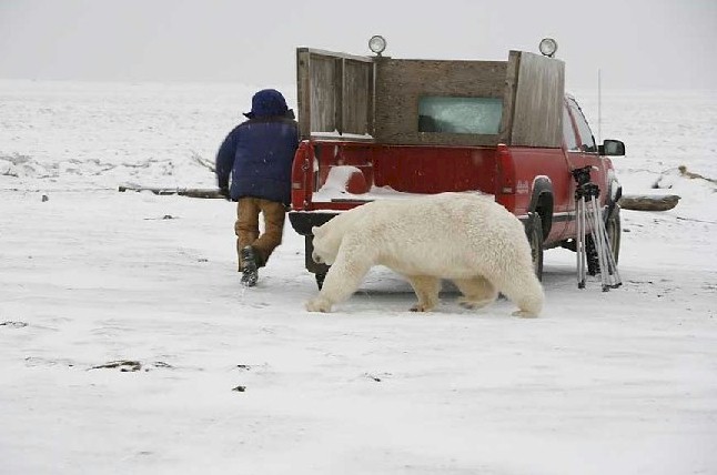
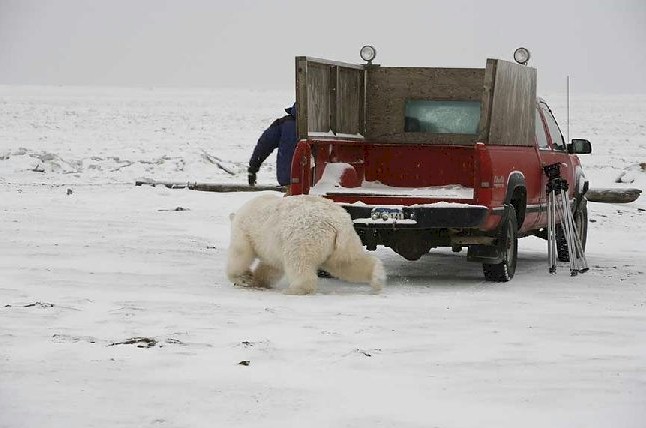
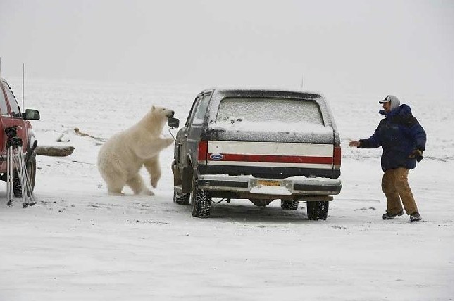
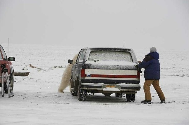
Don't Feed the Bears

One of my brothers forwarded this to me with the caption: “Isn’t it comforting to know that when you are about to become a bear’s breakfast, your buddy is standing there taking photos?”

Submitted Article on Tropical Troposphere Trends

Yesterday Ross and I submitted an article to IJC with the following abstract:

A debate exists over whether tropical troposphere temperature trends in climate models are inconsistent with observations (Karl et al. 2006, IPCC (2007), Douglass et al 2007, Santer et al 2008). Most recently, Santer et al (2008, herein S08) asserted that the Douglass et al statistical methodology was flawed and that a correct methodology showed there is no statistically significant difference between the model ensemble mean trend and either RSS or UAH satellite observations. However this result was based on data ending in 1999. Using data up to the end of 2007 (as available to S08) or to the end of 2008 and applying exactly the same methodology as S08 results in a statistically significant difference between the ensemble mean trend and UAH observations and approaching statistical significance for the RSS T2 data. The claim by S08 to have achieved a “partial resolution” of the discrepancy between observations and the model ensemble mean trend is unwarranted.

Attached to the article as Supplementary Information was code (of a style familiar to CA readers) which, when pasted into R, will go and collect all the relevant data online and produce all the statistics and figures in the article. In the event that Santer et al wish to dispute or reconcile any of our findings, we have tried to make it easy for them to show how and where we are wrong, rather than to set up pointless roadblocks to such diagnoses.

We only consider the comparison between the model ensemble mean trend and observations (the Santer H2 hypothesis). In our discussion, we note that we requested the collated monthly data used by Santer to develop his H1 hypothesis and that this request was refused, attaching the correspondence as supplementary information. Had the H1 data been available when the file was open, we would have analyzed them, but there weren’t, so we didn’t. The results for the H2 hypothesis are interesting in themselves.

We noted that an FOI request to NOAA had been unsuccessful, that the publisher of the journal lacked policies to require the production of data and that an FOI to the DOE was pending. We urged the journal to adopt modern data policies. With all the problems for the new US administration, the fact that they actually turned their minds to issuing an executive order on FOI on their first day in office suggests to me that DOE will produce the requested data. A couple of readers have taken the initiative of writing DOE expressing their displeasure with Santer’s actions as well and they think that the data might become available relatively promptly. Personally I can’t imagine any sensible bureaucrat touching Santer’s little campaign with a bargepole. I’ve long believed that sunshine would cure this sort of stonewalling and obstruction and I hope that that happens.

Update (Jan 27): Events are moving right along as I discovered when I started going through today’s email. In last week’s snail mail, I received a letter dated Dec 10 from some arm of the U.S. nuclear administration (to which Santer’s Lawrence Livermore belongs) acknowledging my FOI request of Nov 14 to the DOE [from memory, I’ll tidy the dates as I don’t have the snail response on hand], saying that it had been in their queue of requests, which are considered in the order in which they are received. The snail seemed especially slow on this occasion. So I wasn’t holding my breath.

Amazingly, in today’s email is a letter from a CA reader saying that the Santer data has just been put online http://www-pcmdi.llnl.gov/projects/msu/index.php (I haven’t looked yet, but will). He sent an inquiry to them on Dec 29, 2008; the parties responsible wrote to him saying that they would look into the matter. They also emailed him immediately upon the data becoming available.

Surprisingly (or not), the same people didn’t notify me concurrently with the CA reader even though my request was almost 6 weeks prior.

A New Metric for Amplification

ABSTRACT: A new method is proposed for exploring the amplification of the atmosphere with respect to the surface. The method, which I call “temporal evolution”, is shown to reveal the change in amplification with time. In addition, the method shows which of the atmospheric datasets are similar and which are dissimilar. The method is used to highlight the differences between the HadAT2 balloon, UAH MSU satellite, RSS MSU satellite, and CGCM3.1 model datasets.

“Amplification” is the term used for the general observation that the atmospheric temperatures tend to vary more than the surface temperature. If surface and atmospheric temperatures varied by exactly the same amount, the amplification would be 1.0. If the atmosphere varies more than the surface, the amplification will be greater than one, and vice versa.

Recently there has been much discussion of the Douglass et al. and the Santer et al. papers on tropical tropospheric amplification. The issue involved is posed by Santer et al. in their abstract, viz:

The month-to-month variability of tropical temperatures
is larger in the troposphere than at the Earth’s surface.
This amplification behavior is similar in a range of
observations and climate model simulations, and is
consistent with basic theory. On multi-decadal timescales,
tropospheric amplification of surface warming is a robust
feature of model simulations, but occurs in only one
observational dataset [the RSS dataset]. Other observations show weak or
even negative amplification. These results suggest that
either different physical mechanisms control
amplification processes on monthly and decadal
timescales, and models fail to capture such behavior, or
(more plausibly) that residual errors in several
observational datasets used here affect their
representation of long-term trends.

I asked a number of people who were promoting some version of the Santer et al. claim that “the amplification behaviour is similar in a range of observations and climate model simulations”, just what studies had shown these results? I was never given any answer to my questions, so I decided to look into it myself.

To investigate whether the tropical amplification is “robust” at various timescales, I calculated the tropical and global amplification at all time scales between one month and 340 months for a variety of datasets. I used both the UAH and the RSS versions of the satellite record. The results are shown in Figure 1 below. To create the graphs, for every time interval (e.g. 5 months) I calculated the amplification of all contiguous 5-month periods in the entire dataset. I took the average of the results for each time interval, and calculated the 95% confidence interval (CI). Details of the method are given in Appendices 2 and 3.

I plotted the results as a curve which shows the average amplification for the various time periods.

Figure 1. Change of amplification with time periods. T2 and TMT are middle troposphere measurements. T2LT and TLT are lower troposphere. Typical 95% CIs are shown on two of the curves. Starting date is January 1979. Shortest period shown is three months. Effective weighted altitudes are about 4 km (~600 hPa) for the lower altitude measurements, UAH T2LT and RSS TLT. They are about 6 km (~500 hPa) for the higher measurements, UAH T2 and RSS TMT.

I love surprises, and climate science holds many … despite the oft repeated claims that the “science is settled”. And there are several surprises in these results, which is great.

1. In both the global and tropical cases, the higher altitude data shows less amplification than the lower altitude. This is the opposite of the expected result. In the UAH data, T2LT, the lower layer, has more amplification than T2, the higher layer. The same is true for the RSS data regarding TLT and TMT. Decreasing amplification with altitude seems a bit odd …

2. In both the global and tropical cases, amplification starts small. Then it rises to about double its starting value over about ten years. It then gradually decays over the rest of the record. The RSS and the UAH datasets differ mainly in the rate of this decay.

3. The 1998 El Nino is visible in every record at about 240 months from the starting date (January 1979).

In an effort to get a better handle on the issues, I examined the HadAt2 balloon record. Here, finally, I see crystal clear evidence of tropical tropospheric amplification.
Continue reading →

Steig’s Silence

Once upon a time, in the mists of time (Feb 2008), long before climate scientists had “moved on”, realclimate featured a post entitled Antarctica is Cold? Yeah, We Knew That, in which Spencer Weart, as noted by Pielke Jr, observed:

. . . we often hear people remarking that parts of Antarctica are getting colder, and indeed the ice pack in the Southern Ocean around Antarctica has actually been getting bigger. Doesn’t this contradict the calculations that greenhouse gases are warming the globe? Not at all, because a cold Antarctica is just what calculations predict… and have predicted for the past quarter century. . .

Bottom line: A cold Antarctica and Southern Ocean do not contradict our models of global warming. For a long time the models have predicted just that.

At AGU in December 2008, Eric Steig gave a preview of his January 2009 article. An RC commenter here reported on this preview as follows:

From http://blogs.nature.com/climatefeedback/2008/12/agu_2008_evidence_that_antarct.html: New research presented at the AGU today suggests that the entire Antarctic continent may have warmed significantly over the past 50 years. The study, led by Eric Steig of the University of Washington in Seattle and soon to be published in Nature, calls into question existing lines of evidence that show the region has mostly cooled over the past half-century.

To which RC coauthor Steig replied (and comments were promptly shut off):

The claim that our result “calls into question existing lines of evidence that show the region has mostly cooled over the past half-century” is wrong though. Wait until the paper is published and I’ll say more.–eric]

Upon recent publication of Steig et al 2009, coauthor Mann stated (also noted up by Pielke Jr):

“Contrarians have sometime grabbed on to this idea that the entire continent of Antarctica is cooling, so how could we be talking about global warming,” said study co-author Michael Mann, director of the Earth System Science Center at Penn State University. “Now we can say: no, it’s not true … It is not bucking the trend.”

Now reasonable people might well interpret that sort of statement as “calling into question existing lines of evidence that show the region has mostly cooled over the past half-century”. Clearly oracles or perhaps goose entrails are required for exegesis of these seemingly contradictory Delphic utterances. Pielke Jr has a little fun with the Team on this, observing:

So a warming Antarctica and a cooling Antarctica are both “consistent with” model projections of global warming.

This elicited a reply from Steig (who seems like pleasant fellow who’s fallen in with a rough crowd over at RC):

I have to admit I cringed when guest writer Weart wrote the article on RealClimate, which I didn’t get a chance to read first. I’m not sure what models he was talking about that said Antarctica should be cooling. A review of the literature would show you (see e.g. Shindell and Schmidt in GRL) that models have been predicting warming.

Fair enough. But this raises the usual problem of the silence of the lambs.

If Steig cringed when he read the Weart article, surely he had an obligation to correct the record at RC. But if you now turn to the thread in question and search ‘Steig’, there is nothing until the final comment (mentioned above.) At no point did Steig record his disagreement with the contents of the RC post. Nor did he record his disagreement when RC coauthors piled on to any commenters who questioned the premises of the Weart post.

Or maybe Steig did write in expressing his disagreement and, like other critics, was censored by Gavin Schmidt. 🙂

Update (Jan 24 4.54 pm): While I was writing this post, Steig added another comment at Pielke Jr

When I said that “I cringed” I don’t mean that I thought there was anything wrong with Spencer’s article. I meant that I thought he wasn’t clear enough that he was referring to the models show a slower warming in Antarctica than e.g. in the Arctic, which was and remains the correct assessment of what the model show. And I suspected that his article would be used in exactly the way Roger Piekle Jr. has used it; to give the impression that scientists are being careless and inconsistent. But as I said above, this is a red herring.

As for why I didn’t make this point at the time, I have a day job. I can’t spend all my time worrying about how blogs on RealClimate may get mis-used and misrepresented by others.

Roger replies in a new post here.

Steig observes that he has a “day job” and can’t worry about how RC gets “misrepresented by others”. But here he is, instantly contesting Roger’s amusement at the RC tangle, not just once but twice. He also had time to make an inline comment closing the past RC thread. So he has time to contest Roger’s supposed miscues, but not to say something at RC about an article that made him “cringe”. Too bad.

Antarctic RegEM

Antarctic: Signy Island - Adelie penguins
Image by mark van de wouw via Flickr

For discussion of new study. by Steig (Mann) et al 2009.

Data:
Data sets used in this study include the READER and AWS data from the British Antarctic Survey. SI Tables 1 and 2 provide listings. They leave out station identifications (a practice that “peer” reviewers, even at Nature, should condemn).

Matches to information at the BAS are complicated by Mannian spelling errors and pointless scribal variations (things like D_10 vs D10, which can be matched manually, but why are the variations there in the first place??)

Anyway, I’ve made collations of the station information in an organized way and collated station and AWS into organized time series (downloaded today) and archived these versions at CA for reader reference. You can download them as follows:

download.file(“http://data.climateaudit.org/data/antarctic_mann/Info.tab”,”temp.dat”,mode=”wb”);load(“temp.dat”)
download.file(“http://data.climateaudit.org/data/antarctic_mann/Data.tab”,”temp.dat”,mode=”wb”);load(“temp.dat”)

If for some absurd reason, you want to analyze them in Fortran or machine language or Excel, you can easily write these things out into ASCII files using R and I’d urge you to learn enough R to do that.

There are references to thermal IR satellite data associated with Comiso. There is a citation to snail literature, but no digital citation. I’ve been unable to locate a monthly digital version of this data – maybe some readers can locate it.

I haven’t been able to locate any gridded output data from the Mannian RegEM analysis. For the PNAS article, Mann et al made a pretty decent effort to archive code and intermediates, but, for the present study, it’s back to the bad old days. No code, no intermediates, not even any gridded output that I can locate.

[Update Jan 23 – Steig says that data will be online next week.]

Station Counts
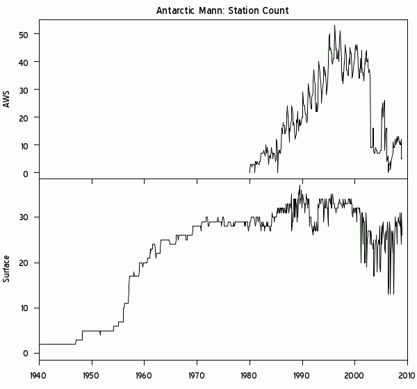
Here’s an interesting little plot from the collation of surface and AWS data. For some reason, there seems to be a sharp decline in AWS counts at the start of 2003 – from 35 at the end of 2002 to 9 at the start of 2003. It seems implausible that this is real though I am not familiar with the data and perhaps it is. Maybe it’s an Antarctic version of GHCN not collecting non-MCDW station data after 1990?

Refs:
Nature 457, 459-462 (22 January 2008) | doi:10.1038/nature07669; Received 14 January 2008; Accepted 1 December 2008.

Eric J. Steig1, David P. Schneider2, Scott D. Rutherford3, Michael E. Mann4, Josefino C. Comiso5 & Drew T. Shindell6

Abstract:
http://www.nature.com/nature/journal/v457/n7228/full/nature07669.html

Full text (pdf): http://thingsbreak.files.wordpress.com/2009/01/steigetalnature09.pdf

SI:

Click to access nature07669-s1.pdf

Methods:
http://www.nature.com/nature/journal/v457/n7228/full/nature07669.html#online-methods

Reblog this post [with Zemanta]

More on Voodoo Correlations

Mann said:

Although 484 (~40%) pass the temperature screening process over the full (1850–1995) calibration interval, one would expect that no more than ~150 (13%) of the proxy series would pass the screening procedure described above by chance alone.

Reader DC said:

Of the 484 proxies passing the 1850-1995 significance test, 342 also passed both sub-period tests (with 341 having r values with matching sign). 111 passed only one of the sub-period tests, and 31 failed both sub-periods.

Let’s think about this a little in terms of statistics. If a “proxy” is a proxy, then it is a proxy regardless of the subperiod. It is not enough to have a “significant” relationship in the 1850-1995 period, it should also have “significant” relationship in the 1850-1949 and 1896-1995 periods (Mann’s late-miss and early-miss periods.)

DC remarked above, in effect, that nearly 30% of the 484 “passing” proxies failed this elementary precaution. I checked this calculation and can confirm it. This can be done as follows.

download.file(“http://data.climateaudit.org/data/mann.2008/Basics.tab”,”temp.dat”,mode=”wb”);load(“temp.dat”)
details=Basics$details; passing=Basics$passing
temp=(passing$whole&passing$latem&passing$earlym);sum(temp)
#342

342 out of 1209 is only 29% (as opposed to Mann’s stated 13% by chance). As observed in September, Mann’s chance benchmark is wrong because his pick two-daily keno method inflates the odds. [As a reader noted, Mann’s 13% is based on the 1850-1995 period and the yield for passing 1850-1995, 1850-1949 and 1896-1995 would necessarily be lower. This goes the other way from pick two daily keno. Autocorrelation is a third benchmarking issue and it doesn;t look to me like Mann’s benchmarks adequately allow for observed autocorrelation.]

I don’t want readers to place any weight on any benchmarks right now other than indicatively, as today I want to look at a different issue: how different proxy classes stand up to this undemanding test. In a given proxy class (ice cores, dendros, speleos, whatever), which proxy classes outperform random picking?

The “best” performer are the Luterbacher series – series which have no business whatever being in a “proxy data sets”. 71 out of 71 Luterbacher series pass the above test. This is not much of an accomplishment since Luterbacher uses instrumental data in his “proxies”. That instrumental data has a high correlation with instrumental data means precisely nothing. You’d think that someone in the climate science “community” would object to this, but seemingly not. The inclusion of these series obviously inflates the count. Without these absurd inclusions, we have 24% of the proxies passing elementary screening ( (342-71)/(1209-71).

“Low-frequency” make up 51 of the 1209 series. Of these 51 series, only 8 series pass the above elementary screening (15.8%). One of these series (Socotra O18- which is non-incidental in M08 reconstructions BTW), fails an additional undemanding test that “significance” have a consistent sign. This leaves 7/51 (13.7%) as being “significant”.

annual=Basics$criteria$annual;
c(sum(!annual),sum(temp&!annual))#51 8

Code 9000 dendro proxies make up over 927 of 1209 M08 proxies. Only 143 pass the above simple test ( 15.4%).

dendro=(Basics$details$code==9000)
c(sum(dendro),sum(temp&dendro)) #[1] 927 143

On the other hand, Briffa MXD proxies (code 7500) have a totally different response: 93 out of 105 (88%) pass M08 screening. This is such a phenomenonal difference from run-of-mill dendro proxies that one’s eyebrows arch a little. Now these aren’t ordinary Briffa MXD proxies. These series were produced in part by Rutherford (Mann) et al 2005 performing RegEM on Briffa MXD data; then M08 truncated the Rutherford Mann MXD versions in 1960 because of the “divergence” problem and replaced actual data from 1960 to 1990 by infilled data, all prior to calculating the above correlation. I haven’t parsed every little turn of Mannian adjustments, but you will understand if I view the statistical performance of this data for now as a little suspect. None of this data is earlier than AD1400 in any event.

I’ll look at the other classes of data (only 55 series left) tomorrow.

realclimate and Disinformation on UHI

In a recent CNN interview discussed at RC here, Joe D’Aleo said:

Those global data sets are contaminated by the fact that two-thirds of the globe’s stations dropped out in 1990. Most of them rural and they performed no urban adjustment. And, Lou, you know, and the people in your studio know that if they live in the suburbs of New York City, it’s a lot colder in rural areas than in the city. Now we have more urban effect in those numbers reflecting — that show up in that enhanced or exaggerated warming in the global data set.

Gavin Schmidt excoriated this claim as follows:

D’Aleo is misdirecting through his teeth here. … he also knows that urban heat island effects are corrected for in the surface records, and he also knows that this doesn’t effect ocean temperatures, and that the station dropping out doesn’t affect the trends at all (you can do the same analysis with only stations that remained and it makes no difference). Pure disinformation.

Later in the comments (#167), an RC reader inquired about UHI adjustments, noting the lack of discusison of this point as follows:

#167/ In all of the above posts there is no mention of the urban heat island effect, nor of the effect of rural station drop out nor of the effect the GISS data manipulation has on surface temperature. Why is that?

To which Gavin replied:

[Response: Because each of these ‘issues’ are non-issues, simply brought up to make people like you think there is something wrong. The UHI effect is real enough, but it is corrected for – and in any case cannot effect ocean temperatures, retreating glaciers or phenological changes (all of which confirm significant warming). The station drop out ‘effect’ is just fake, and if you don’t like GISS, then use another analysis – it doesn’t matter. – gavin]

Neither CRU nor NOAA have archived any source code for their calculations, so it is impossible to know for sure exactly what they do. However, I am unaware of any published documents by either of these agencies that indicate that they “correct” their temperature index for UHI effect (as Gavin claims here) and so I’m puzzled as to how Gavin expects D’Aleo to be able to “know” that they carry out such corrections. And as to GISS adjustments, as we’ve discussed here in the past (and I’ll review briefly), outside the US, they have the odd situation where “negative UHI adjustments” are as common as “positive UHI adjustments”, raising serious questions about whether the method accomplishes anything at all, as opposed to simply being a Marvelous Toy. Continue reading →

Jones et al 2009: Studies Not "Independent"

One of the ongoing Team mantras has been that the Mann hockey stick has been supported by a “dozen independent studies”. Obviously, I’ve disputed the claim that these studies are “independent” in any non-cargo cult use of the term “independent”. A new article by Jones and multiple coauthors (Holocene 2009) comments on this issue. Continue reading →

Rain in Maine Falls Mainly in the Seine

A blog article here reviews the “standing joke” of Mann’s stubbornness in refusing to correct the wrong locations of MBH98 in the recent Mann et al 2007 network, where, as I observed, the prior errors are perpetuated without apology, even though the incorrectness of the locations has long been known to Mann. In a routine google, I noticed that there are even “rain in Maine” T-shirts , though the vendors have, for some reason, used a Parisian scene.