Toeplitz Matrices and the Stahle Tree Ring Network

One of the most ridiculous aspects and most misleading aspects of MBH (and efforts to rehabilitate it) is the assumption that principal components applied to geographically heterogeneous networks necessarily yield time series of climatic interest.

Preisendorfer (and others) state explicitly that principal components should be used as an exploratory method – and disavowed any notion that merely passing a Rule N test imbued a time series with magical properties.

In primitive societies, there is a “correct” order for magical incantations and woe betide anyone who dares to question the authority of the witch doctors. We see this with the recent discussion at Tamino’s of Rule N: total disregard for any need to establish the scientific veracity of a relationship between ring widths and temperature and replacement of such investigation by incantations that certain relatively arbitrary methods are “correct” or “proper”, using the language of ritual or magic rather than science.

There is much that needs to be said on this topic and I will do so next week.

Today, I want to discuss something very interesting that arose in the discussion of the Stahle SWM network – an “uncontroversial” network, but which may have great utility in understanding the properties of principal components applied to geographically heterogeneous tree ring networks.

I’d plotted up barplots of the Stahle SWM network eigenvectors and, at the suggestion of a reader, eigenvector contour maps. These plots had several extremely interesting properties which are connected with known properties of Toeplitz matrices – hence the title – which, in turn, give some considerable insight into the meaning of principal components applied to such networks – a topic conspicuously lacking in all literature to date.. Continue reading

Tamino and the "Adjusted" Gaspé Data

Tamino, in his continuing effort to bring every one of Mann’s questionable practices back into the light of day, has stumbled into the treeline11.dat series, which he proclaims triumphally in his most recent post as having a hockey stick shape. This is none other than the notorious Gaspé cedar series, which was analyzed at length in MM2005 (EE).

Tamino purports to be a data analyst capable of criticizing our published corpus. It’s pretty discouraging when a “data analyst” can’t even figure out that treeline11.dat is the Gaspé series and that there are many problems with it

But hey, if Tamino wishes to pick at these scabs, that’s more than fine with me. The Gaspé series illustrates the problems with Team proxy reconstructions, just as well as the bristlecones. Here are some of the problems.

First and this is a big problem. Mann adjusted the treeline11.dat series without disclosing the adjustment. In the entire corpus of 415 MBH series, only one series was extended at its beginning to enable it to avoid a cut-off point (and include it in an earlier network.) You guessed it – the Gaspé series in the AD1400 network, which was a troublesome section of the reconstruction. It is my opinion that the extension of the Gaspé series was not accidental and was done in order to affect results in the AD1400 network. Unique “adjustments” like this are the sort of thing that financial accountants take great exception to. Rob Wilson confirmed to me that “such extrapolation is not a standard approach in the tree-ring community.”

Second, the unique adjustment was not disclosed in the MBH98 footnotes. Worse, the start date of this series was actually misrepresented in the original supplementary information, which listed the series as starting at the “adjusted” start date rather than the true start date. We only noticed the extrapolation when we compared the Mann version to original data. We noted this in MM 2003, but were not then fully aware of the impact.

Third, in the early portion of the Gaspé chronology, there is only one tree – a point that was widely publicized back in 2005. Standard chronological methods require a minimum of 5 cores and preferably more. The early portion of the Gaspé chronology did not meet quality control standards. Again, Wilson confirmed that chronologies should not be used in periods where there is only a single core. If Mann wanted a site from the Jacoby network for his AD1400 network, then one was readily available without having to “adjust” anything. The archived Sheenjek River version goes back to 1186; instead of using this archived version, Mann used a “grey” version. Sheenjek does not have a HS shape. Mann et al 2007 uses the same network as MBH98, not removing the “adjustment” even after it’s been discovered and not using the updated Sheenjek version.

Fourth, the Gaspé series is a cedar chronology. There is no botanical evidence that cedars respond linearly to warmer temperatures. World experts on cedar are located at the University of Guelph, Ross McKitrick’s university. Ross and I had lengthy discussions with these cedar experts about this chronology – they said that cedars like cool and moist climate.

Fifth, the Gaspé chronology was never published in formal literature. There was an informal description in Natural Areas Journal, where the HS shape was observed – with the caution that this shape would have to be confirmed in other sites, mentioning pending cedar sites in Maine and Michigan. Neither of these sites had a HS shape. There is another long cedar chronology in the ITRDB (Lac Duparquet – cana106). This series was listed in the original SI as being used, but was not used, as later admitted in the Corrigendum. It does not have a HS shape.

Sixth, and this is very troubling: an update to Gaspé was done in the early 1990s – the update did not get a HS shape (shown below). This update was never published. I happened to obtain a copy of the update which was shown at CA here. The updated version of the Gaspé series does not have a HS shape. It has never been shown publicly except here at CA. Jacoby and d’Arrigo refused to provide me with either the updated chronology or with the measurement data. D’Arrigo refused to provide the updated information on the basis that the older version was “probably superior with regards to a NH signal”. The updated Gaspé information was taken over 15 years ago and has never been archived. When I objected to NSF, which funded the collection of the update, they took no action to require Jacoby and D’arrigo to archive the missing data.

Seventh, none of Cook, Jacoby or D’Arrigo would provide this information on the location of the Gaspé cedars when I inquired, saying that I wished to re-sample the site. They claimed that the collection was done prior to GPS and that they didn’t know where it was.

The Gaspé series demonstrates in one nice package many different aspects of the problems with Team reconstructions. And yes, that’s Tamino treeline11.dat. Again I refer readers to MM 2005(EE) where the problems with the Gaspé series are discussed at length. Again, Tamino has inaccurately represented the research record.

Rule N and Weighted Regression

Today’s post, which has a forbidding title, contains an interesting mathematical and statistical point which illuminates the controversy over how many PCs to retain. In my re-visiting the totally unknown corner of Mannian methodology – regression weights and their determination – I re-parsed the source code, finding something new and unexpected in Mannian methodology and resolving a puzzling issue in my linear algebra.

The key to the idea is very simple. After creating a network of proxies, Mann does what are in effect two weighted regressions: first, a calibration regression in which the proxies are regressed against the temperature PCs weighted by their eigenvalues; second , an estimation regression in which the reconstructed temperature PCs are estimated by a weighted regression in which different weights are assigned to each proxy. These weights ranged from 0.33 to 1.5.

Now there’s an interesting aspect to Mann’s implementation of the weights using SVD, which has taken me a long time to figure out. After a new push at parsing the source code, I’ve determined that the code actually implements weighting by the square of the weights. I’m going to do a very boring post on the transliteration of these weighting calculations from Mannian cuneiform into intelligible methodology in a day or two.

The effective weighting thus varies from 0.11 to 2.25 (a range of over 20) – with the largest weight being assigned to the Yakutia series. This is amusing, because Yakutia is an alter ego for the Moberg Indigirka series which has a very elevated MWP – we discussed this in connection with Juckes. Use of the updated long Yakutia-Indigirka series will have a dramatic impact on MBH99 as well as Juckes – something that I’d not noticed before.

In the AD1400 network, the sum of squares of all 22 weights is 12.357, of which the NOAMER network accounts for about 16% of the total weight.

How were these weights determined? No one knows. Actually I challenge Tamino or anyone else to locate these weights. Weighted regression is not mentioned in MBH98 itself. Indeed, MBH98 contains an equation for this step which clearly fails to show that weighting was done. They are not discussed in the Corrigendum but weights are given in the Corrigendum SI in files http://www.nature.com/nature/journal/v430/n6995/extref/PROXY/data1400.txt. In the source code provided to the House Energy and Commerce Committee, the weights are referred to in the code by the variable weightprx.

Weights are mentioned in passing in Wahl and Ammann, who stated incorrectly that:

A second simplification eliminated the differential weights assigned to individual proxy series in MBH, after testing showed that the results are insensitive to such linear scale factors.

and

Additionally, the reconstruction is robust in relation to two significant methodological simplifications-the calculation of instrumental PC series on the annual instrumental data, and the omission of weights imputed to the proxy series. Thus, this new version of the MBH reconstruction algorithm can be confidently employed in tests of the method to various sensitivities.

The argument below shows exactly how incorrect these claims are and how theses claims are inconsistent with Wahl and Ammann’s own confirmation of results using 2 and 5 PCs.


Weights and PC Retention

To illustrate the connection between weights and PC retention, showing how PC retention can be viewed as a special form of regression weighting, let’s construct a network using centered PCs with 5 PCs included. Perhaps through Rule N (even if it wasn’t used in MBH98, it’s not an implausible rule.)

Here’s how special choices of weights yield the two cases that have been at issue so far. If you give weights of (1,1,0.001,0.001,0.001) to the 5 PCs, then you’ll get a result that is virtually identical to the retention of only 2 PCs, while if you give equal weights to the 5 PCs, then you’ll get a result that looks like the Stick – heavy weighting on the bristlecones. Wahl and Ammann agree that you get different results using 2 and 5 covariance PCs. So obviously the selection of weights can “matter” – their own calculations confirm this. They happened to show one calculation where the two choices didn’t matter much, but that hardly rises to the standard of mathematical proof. It’s amazing how low the standards of reasoning are in this field.

If you assign equal unit weights to all 5 PCs in the network now represented by 5 PCs instead of 2 PCs, you also increase the proportion of weighting assigned to the NOAMER network relative to all weights. With two PCs, the NOAMER network had about 16% of the weights, but, if 5 PCs are each assigned equal weight, then the proportion of weight increases from 2/12.357 to 5/15.357 or nearly doubles.

Let’s suppose for a moment that there was a reason why Mann allocated 16% of the total weights to the NOAMER network. Perhaps it wasn’t clearly articulated but one can’t exclude the possibility that there was a reason. Why would the proportion assigned to this network increase because of the decision to increase the number of PCs used to represent the network? Mann has changed this aspect of his methodology. On the basis that this network should represent 16% of the total weight, then the weight allocated to all 5 PCs should still amount to 16% of the total weight. Instead of equal unit weights, the 5 PCs should be assigned lower weights.

There’s another weighting issue which reflects the reduced proportion of total variance accounted for by a PC4 (and is a pleasing and rational way of dealing with the frustration that a PC4 should dominate the subsequent regression.) In Mann’s calibration, he weighted the temperature PCs by their eigenvalues. Now this procedure is undone by the subsequent rescaling (hey, this is Mann we’re talking about), but the idea of weights by eigenvalues is not a bad one.

So a plausible implementation for the tree ring network would be to weight each tree ring PC by its eigenvalue so that the more important PCs were weighted more heavily, requiring also, as in the prior paragraph, that the total weights be apportioned so that the network still accounts for 16% of total weight. If this quite plausible procedure is done, then the weights assigned to the Graybill bristlecones are reduced substantially – so that the resulting recon is only marginally different from the reconstruction using 2 PCs as shown below:

weight21.gif

I absolutely don’t want readers to get the impression that any of these squiggles mean anything. They are just squiggles. The MBH squiggle gets a HS shape from higher weighting of Graybill bristlecone chronologies. As I’ve said over and over, the Graybill Sheep Mt chronology was not replicated by Ababneh and all calculations involving the Graybill Sheep Mt chronology (including MBH, Mann and Jones 2003, Mann et al 2007, Juckes, Hegerl etc) should be put in limbo pending a resolution of the Sheep Mt fiasco.

Today I’m just making an appealing mathematical point – differences between the number of retained PCs can and should impact the weights in the weighted regression. The statement by Wahl and Ammann that these weights don’t matter – as a mathematical point – is, in Tamino’s words, “just plain wrong”. Purporting to salvage MBH by increasing the number of retained PCs without reflecting this in the overall weight assigned to the network increases the proportion of weight assigned to the network – in this case dramatically.

If the overall weight of the network is left unchanged and the PCs additionally weighted in proportion to their eigenvalues, the net result does not yield a HS using AD1400 proxies.

Bilge in Tamino's Canoe

In order to illustrate a useful application of principal components, Tamino showed coordinate systems for the motion of a canoe. In the context of MBH, it would have been more instructive to show how principal components apply to tree ring networks than to canoes. In such a context,a non-Mannian centered PC1 will typically show some sort of weighted average and lower PCs will show contrasts, which feature increasingly trivial and local contrasts. I’ll show this in connection with the Stahle SWM network used in MBH98, where there is relatively little difference between Mannian and centered PCs and which will give readers a flavor of exactly how little utility the lower order PCs have.

Readers may also consider the following assumption underlying MBH:

Implicit in our approach are at least three fundamental assumptions. (1) The indicators in our multiproxy trainee network are linearly related to one or more of the instrumental training patterns. In the relatively unlikely event that a proxy indicator represents a truly local climate phenomenon which is uncorrelated with larger scale climate variations, or represents a highly nonlinear response to climate variations, this assumption will not be satisfied.

As you examine the weights of different Stahle/SWM PCs, reflect on whether MBH have successfully excluded the possibility that (say) the Stahle PC8 (or for that matter the PC3, PC2 or PC1) might simply be some local noise. Continue reading

Principal Components and Tree Ring Networks

I’m finding some benefit to having spent some time on station histories prior to my present re-visit to Mannian proxies. Digging into the handling of station histories gives some interesting perspectives on network handling that are worth considering for tree ring networks.

For example, assume for a moment that North American tree ring chronologies used in MBH98 actually were little thermometers. Yeah, yeah, I know all the problems with them. But let’s suppose that they actually were little thermometers, noisy little station histories going back hundreds of years. What would Phil Jones or Hansen or USHCN would do if they had dozens of North American station histories going back 600 years?

You know right away what they’d do: they’d lay out a grid over North America; they’d allocate each station to its respective gridcell; they’d form anomaly series by subtracting the mean over a common interval, take an average over each gridcell of available records and then take an average over all the gridcells.

Would they do principal components on the raw geographically inhomogeneous station data? Of course not. What meaning could one possibly attach to geographically inhomogeneous station data? Would they do stepwise principal components when there was missing data? The mind boggles at CRU doing something like that.

As an exercise, I thought that it would be interesting to do a CRU-type “gridcell history” for Mann’s NOAMER network.

An interesting issue arose in starting this – one that we reflected on a bit in MM2003, but haven’t discussed much. The MBH “NOAMER” network is actually a subset of about 75% of the North American tree sites used in MBH98. The first figure shows a location map of all the tree ring sites mentioned in the original MBH SI, color coded to illustrate the following.

The pink dots show the Graybill bristlecone sites in the AD1400 network – the sites that so much controversy attaches to. Geographically they obviously in a restricted range in the US southwest; the blue dots show the rest of the 70 sites in the AD1400 NOAMER network; the green dots show the other 141 sites used in later steps of the NOAMER network; the cyan dots show the Jacoby network (each site being used individually in MBH), with the Gaspe site used in the AD1400 regressions shown a little larger. The brown dots show the Stahle SWM and Stahle OK networks, many sites being between “NOAMER” sites and a couple of sites in the Four Corners area being used in both networks. The red dots show the sites listed in the original SI but not used in the NOAMER network – for reasons that have been never been properly explained. Their non-use was admitted in the MBH Corrigendum , which provided a false excuse for their non-use:

These series, all of which come from the International Tree Ring Data Bank (ITRDB), met all the tests used for screening of the ITRDB data used in ref. 1 (see ref. 5), except one—namely, that in 1997, either it could not be ascertained by the authors how these series had been standardized by the original contributors, or it was known that the series had been aggressively standardized, removing multidecadal to century-scale fluctuations.

This is untrue. Some of the excluded series (red) were Schweingruber series; all sorts of Schweingruber series were used in MBH98 and the excluded series came from identical publications as included series. This was pointed out to Nature, but they didn’t care. When I plotted this up, I noticed two red dots in Alberta – these are both locations where Rob Wilson has worked; one of the series was used in Esper et al 2002.

noamer3.gif
Figure 1. North American tree ring sites used in MBH98.

Anyway, continuing with my development of a “station history” type procedure. As a test, I did one on the MBH NOAMER network without worrying about exclusions and Stahle and that sort of stuff. I standardized the series on 1613-1900 as a long period over which the MBH NOAMER network has values to the beginning. My guess is that standardization with 1613-1970 values wouldn’t make much difference and I’ll probably do this calculation as well if I pursue this any more.

I allocated all the series to 5×5 Jones-style gridcells and averaged all available standardized chronologies within each gridcell, thereby forming a gridded network of 31 gridcells. I then calculated an annual average over all available values using a truncated mean (not using the two extreme values on either end). This yielded the following North American Tree Ring Index, shown to 1980 the final year of MBH tree ring calculations.

I’ve marked a few years with extreme values. 1934, known to be an exceptionally hot year in the U.S., had the lowest “Tree Ring Index” in the period 1880-1980. 1946 had the highest. The decade in the 1840s had exceptionally low growth – something that we also noticed in our Almagre samples. There’s certainly no hockey-stick in this Tree Ring Index.

noamer4.gif
Figure 2. North American Tree Ring Index

Intrigued by this result, I download a CRU gridded temperature history (using HadCRU2 for this since it’s a little more contemporary to MBH98) and calculated the correlation of the gridded growth index to CRU temperature history for each gridcell. I then made a contour map using the akima package that I had previously used for station history plots. For this calculation, I re-did the grids using all the available stations – Stahle, Jacoby, excluded sites.

noamer55.gif
Figure 3. Correlation to Temperature

Obviously one feature that sticks out like a sore thumb: the gridded growth histories in the U.S. Great Plains are negatively correlated to temperature. It looks to me like the core of this negative correlation is pretty near Crawford, Texas.

There’s a strip along western Canada that shows positive correlation. If you look back at the location map, you’ll see that this has mostly been filled in by interpolation as there are no MBH network stations. Also something curious – this positive correlation area is bounded at either end by stations that Mann deleted from his network, stations that weren’t used.

So we can see one reason why a station history approach doesn’t work very well – we don’t know whether our little thermometers are reading up or down. For example, suppose that a new treasure trove of instrumental measurement data decoded from Aztec or Maya glyphs were delivered to Phil Jones – the only problem was that you didn’t know whether the numbers ran up or down. Even CRU wouldn’t just dump all this data into their data base and hope that some algorithm could sort it out. Before the Aztex instrumental data was incorporated into station history data bases, one would hope that some sort of technical study would be done showing how to convert the Aztec instrumental data into modern terminology, demonstrating which direction was up in their nomenclature and what their scale was? Tree rings should be no different.

And what if Phil Jones found that some of the Aztec data was actually instrumental precipitation measurements. Would he just dump that into his data base and hope that it improved things? That maybe there was a teleconnection between Aztec instrumental precipitation and temperatures in some other part of the world. As soon as you even write this down, you realize that someone would first have to demonstrate that there was a solid relationship between modern measured precipitation in the Yucatan and modern instrumental temperatures in (say) Timbuktu or wherever, and demonstrate that this information actually aided in the estimate in a way that rose above data mining before assuming that Aztec instrumental precipitation measurements contained useful information for temperature reconstructions.


Comparison to the MBH PC1

The above graphic showing the relationship of gridded tree ring growth and gridcell temperature may provide a helpful perspective on bristlecones and the Mannian PC1 (or the PC4 or whatever).

In the graphs below, I show the geographical properties of the MBH weighting so that readers can appreciate how the locations of the famous MBH PC1 fit in the above map. On the left I’ve done a contour map in which each value of the MBH98 PC1 eigenvector is located spatially at its site. I’m experimenting a little with this still. On the right is a plot in which the weight of each site is shown by the area of the dot. Graybill bristlecone/foxtail chronologies are shown in red; all others are shown in green. The key Sheep Mt site is near the CA-NV border in California.

The Graybill bristlecone chronologies (especially the key Sheep Mountain chronology) are, on this coarse scale, in areas where there is neither a strong positive nor strong negative correlation of growth to temperature – in a shoulder zone. This agrees with site specific analyses, which show little positive correlation of bristlecone growth to temperature (nor negative correlation.)

For someone that’s looked at a lot of geophysical maps in my life, the supposed occurrence of bristlecone chronologies measuring world climate in such a shoulder zone raises red flags. Why should a site chronology in a U.S. shoulder zone have a loud response to world climate, when the chronology (and the gridded “station history”) have negligible correlation. One would surely investigate the possibility of some artifact in the Graybill chronology. Given Linah Ababneh’s failure to replicate the Graybill chronology, the alarm bells should be ringing even in Mann-world.

noamer31.gif pcsht41.gif

UPDATE: Woodhouse and Overpeck (BAMS 1998) show the following comparison between a tree ring reconstruction of drought and observed Palmer PDSI in 1934 – a year of low overall growth. It’s not that relevant specialists are unaware of the connection between U.S. tree rings and drought. Exactly why none of them ever commented on these issues in connection with MBH is something you’d have to ask them.

noamer16.jpg
From Woodhouse and Overpeck BAMS 1998

Here’s the MBH98 PC1 (bristlecones) again marking 1934. Given that bristlecone ring width are allegedly responding positively to temperature, it is notable that the notoriously hot 1934 is a downspike.
noamer47.gif

Svalgaard #4

Continued from here.

Unthreaded #32

The CA server has been a bit balky this week, so I want to see if the volume of info on unthreaded #31 (768 comments) might have something to do with it by starting a new thread to see if the issues abate.

Also per John A, can I recommend that contributors to Unthreaded conversations use the message board also?

A Challenge to Tamino: MBH PC Retention Rules

Today I wish to re-visit an issue discussed in one of the very first CA posts: did MBH98 actually use the PC retention rules first published in 2004 at realclimate here and described both there and by Tamino as “standard” selection rules.

Much of the rhetorical umbrage in Tamino’s post is derived from our alleged “mistakes” in supposedly failing to observe procedures described at realclimate. As observed a couple of days ago, Tamino has misrepresented the research record: both our 2005 articles observed that the hockey stick shape of the bristlecones was in the PC4. In MM 2005 (EE), we observed – citing the realclimate post as Mann et al 2004d:

If a centered PC calculation on the North American network is carried out (as we advocate), then MM-type results occur if the first 2 NOAMER PCs are used in the AD1400 network (the number as used in MBH98), while MBH-type results occur if the NOAMER network is expanded to 5 PCs in the AD1400 segment (as proposed in Mann et al., 2004b, 2004d ). Specifically, MBH-type results occur as long as the PC4 is retained, while MM-type results occur in any combination which excludes the PC4. Hence their conclusion about the uniqueness of the late 20th century climate hinges on the inclusion of a low-order PC series that only accounts for 8 percent of the variance of one proxy roster.

Mann, M.E., Bradley, R.S. and Hughes, M.K., 2004d. False Claims by McIntyre and McKitrick regarding the Mann et al. (1998) reconstruction. Retrieved from website of realclimate.org at http://www.realclimate.org/index.php?p=8.

In MM2005 (EE), we observed correctly that you got a HS-shaped reconstruction if you use 5 PCs (including the bristlecones in the PC4), while you don’t get one if you use 2 PCs. (We considered many other permutations in MM2005 (EE), including correlation PCs; Tamino’s not the first person to criticize us without properly reading our articles.) Despite the above clear statement, Tamino distorted the research record by falsely alleging that we had failed to consider results with 5 PCs:

When you do straight PCA you *do* get a hockey stick, unless you make yet another mistake as MM did. .. When done properly on the actual data, using 5 PCs rather than just 2, the hockey stick pattern is still there even with centered PC — which is no surprise, because it’s not an artifact of the analysis method, it’s a pattern in the data.

Here Tamino, as he acknowledges, relies heavily on Mann’s early 2005 realclimate post where Mann stated: :

MM incorrectly truncated the PC basis set at only 2 PC series based on a failure to apply standard selection rules to determine the number of PC series that should be retained in the analysis. Five, rather than two PC series, are indicated by application of standard selection rules if using the MM, rather than MBH98, centering convention to represent the North American ITRDB data. If these five series are retained as predictors, essentially the same temperature reconstruction as MBH98 is recovered (Figure 2).

So what exactly is this “mistake” that we are supposed to have made? We said that you got a HS reconstruction with 5 PCS; so did Mann and Tamino. We said that you didn’t get a HS reconstruction with 2 PCs, so did Mann and Tamino. Their argument, as I understand it, is that it is a “mistake” to do a reconstruction with 2 PCs rather than 5 PCs, as 5 PCs are mandated by “standard selection rules”.

I’ve reviewed what Preisendorfer and others have said about determining “significance” of PCs – that PC analysis is merely exploratory and Rule N (or similar rules) merely create a short list of candidate patterns; they do not themselves establish scientific significance. As Preisendorfer said, there is no “royal road” to science. Someone somewhere has to do the grunt work of showing that the PC4 has scientific validity as a temperature proxy, a Rule N analysis can’t do that.

But today I want to discuss something quite different and something that has really annoyed me for a long time. For all the huffing and puffing by Mann and Tamino about Preisendorfer’s Rule N being a “standard selection rule” or a “correct” way of doing things, Mann failed to produce the source code for the Preisendorfer tree ring calculations when asked by the House Energy and Commerce Committee for MBH98 source code, even though it was a highly contentious issue where implementation errors had already been alleged.

Worse, as shown below (re-visiting a point made in early 2005), it is impossible to reproduce the observed pattern of retained PCs shown for the first time in the Corrigendum SI of July 2004. MBH98 itself made no mention of Rule N in connection with tree ring networks, referring instead to factors such as “spatial extent” which have nothing to do with Rule N:

Certain densely sampled regional dendroclimatic data sets have been represented in the network by a smaller number of leading principal components (typically 3–11 depending on the spatial extent and size of the data set). This form of representation ensures a reasonably homogeneous spatial sampling in the multiproxy network (112 indicators back to 1820)

In fact, when one re-examines the chronology of when Rule N was first mentioned in connection with tree rings, it is impossible to find any mention of it prior to our criticism of Mann’s biased PC methodology (submitted to Nature in January 2004) and Mann then noticing that the hockey stick shape of the bristlecones was in the PC4, a point first made in Mann’s Revised Reply to our submission, which presumably was submitted around May 2004. The Supplementary Information 1 to that submission was substantially identical to the later realclimate post (this post itself being one of the very first dated posts, actually preceding the start-up of realclimate on Dec 1, 2004 – evidencing perhaps a little too much interest in the matter on their part, something that is worth noticing. )

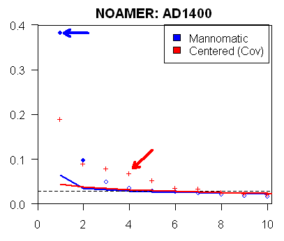
I’ve been substantially able to replicate the methodology illustrated in the realclimate post and I’ve applied the methodology to all other MBH98 network/step combinations, resulting in some disquieting inconsistencies. The figure below shows on the left the realclimate Rule N calculation for the AD1400 NOAMER network. The 4th red + sign marks the eigenvalue of the bristlecone PC4 upon which the MBH98 reconstruction depends in this period. The red + signs show eigenvalues using a centered (covariance) calculation; the blue values are using Mannian PCs. The two lines show simulated results generating random matrices based on AR1 coefficients. On the right is my emulation of this calculation – which, as you can see, appears to be identical. The eigenvalue information shown here is completely consistent with the information in MM 2005 (GRL) and MM2005 (EE).

The blue arrow shows the eigenvalue of the bristlecone-dominated PC using Mannian methods; the red arrow show the eigenvalue using a centered calculation. These results were reported in MM2005 (GRL) where we stated that explained variance of the bristlecones wsa reduced from 38% (the blue arrow) to 8% (the red arrow) and that the bristlecones were not the “dominant component of variance” in the North American network, as previously claimed by Mann et al – an impression that they would obviously have been given by their incorrect PC calculation. So when they say that the error didn’t “matter”, it certainly mattered when they said that this particular shape was the “dominant component of variance” or the “leading component of variance”, claims that they made in response to our 2003 article.

 preise1.gif  tamino50.gif

Caption to realcimate figure and MBH 2004 Nature submission: FIGURE 1. Comparison of eigenvalue spectrum for the 70 North American ITRDB data based on MBH98 centering convention (blue circles) and MM04 centering convention (red crosses). Shown is the null distribution based on simulations with 70 independent red noise series of the same length with the same lag-one autocorrelation structure as the actual ITRDB data using the centering convention of MBH98 (blue curve) and MM04 (red curve). In the former case, 2 (or perhaps 3) eigenvalues are distinct from the noise floor. In the latter case, 5 (or perhaps 6) eigenvalues are distinct from the noise floor. The simulations are described in “supplementary information #2”.

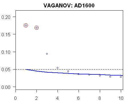
Now for some fun. The figure below shows the calculations for two other MBH98 network/step combinations, illustrating here Mannian PC results for comparison to actual retention. On the left is a calculation for the Vaganov AD1600 network where 2 PCs were retained (retained PCs are circled.) PCs 3,4 and 5 were not retained, but all are “significant” according to the Rule N supposedly used in MBH98. In fact, the unused PC3 here is surely more “significant” than the covariance PC4 which Mann now claims under the algorithm illustrated at realclimate.

On the right is another network – Stahle.SWM AD1750, showing an opposite pattern. In this case, MBH retained nine PCs although only three are “significant” under the realclimate version of Rule N. This is also a relatively small network (located in southwestern U.S. and Mexico and inexplicably excluded from the NOAMER network with which it somewhat overlaps.)

 tamino48.gif  tamino49.gif

Note: The dotted line additionally shows the 2/M “rule” that was noticed in the examination of the source code in connection with Mann deciding how many “climate fields” to retain. It’s not mentioned anywhere but is also illustrated here for convenience.

It seems quite possible to me that the Rule N version illustrated at realclimate was not actually used in MBH98. The first surfacing of the realclimate algorithm in the present form came only after Mann realized that the bristlecone hockey stick really did occur in the PC4 and was not the “dominant component of variance”. There is no contemporary evidence that it was used and there is no source code proving its use. Both Mann and Nature refused to provide details back in 2003 and 2004. The actual pattern of retained PCs cannot be reproduced according to the way that I’ve implemented the realclimate algorithm. As I said earlier, I’m not sure why Tamino has decided to re-open these particular scabs. In Mann’s shoes, I would have left this stuff alone.

The question for Tamino. Which is incorrect: the information on retained PCs at the Corrigendum SI? Or the claim that the algorithm illustrated at realclimate was used in that form in MBH98? If there is some other explanation, some way of deriving the Vaganov AD1600 and Stahle/SWM AD1750 using the realclimate algorithm, please show how to do it. I’ll post up data and code for my implementation to help you along. C’mon, Tamino. You’re a bright guy. Show your stuff.

UPDATE: Willis Eschenbach reports below in a comment that he has examined also examined these calculations and results and also concludes that MBH98 did not use Rule N.

NOTE: Just in case Tamino says that …sigh… it’s too much work, here’s my script. The functions used for the calculations are in http://data.climateaudit.org/data/mbh98/preisendorfer.functions.txt and can be analyzed there in case there are any defects; the collated information is http://data.climateaudit.org/data/mbh98/preisendorfer.info.dat and the tree ring networks are in http://data.climateaudit.org/data/mbh98/UVA. These can be read into an R session as follows:

source(“http://data.climateaudit.org/data/mbh98/preisendorfer.functions.txt”)
target=read.table(“http://data.climateaudit.org/data/mbh98/preisendorfer.info.dat”,sep=”\t”,header=TRUE)
mbhdata=”http://data.climateaudit.org/data/mbh98/UVA”

The Stahle 1750 graphic can be produced using this command (and the functions show the calculation):

plotf(7)

The Vaganov 1600 example can be produced as follows:

plotf(19)

The North American comparison can be done as follows:

i=8;x=preis_emulation(network=target$network[i],step=target$period[i])
test=preis_emulation(network=target$network[8],step=target$period[8],method=”covariance”)
#Do Plot illustrated at CA
ylim0=1.2*max(x[1,]);M=nrow(x)
plot(1:M,x$preis,type=”l”,lwd=2,col=4,las=1,ylab=””,xlim=c(0,10.2),xlab=””,xaxs=”i”,ylim=c(0,.4),yaxs=”i”)
points(1:M,x$lambda,col=4)
abline(h=2/M,lty=2)
points(1:M,test$lambda,col=2,pch=”+”)
lines(1:M,test$preis,col=2,lwd=2)
title(main=paste(target$network[i],”: AD”,target$period[i],sep=””) )
temp=( (x$lambda-x$preis)>0); target$preis[i]=sum(temp)
L=target$series[i];points(1:L,x$lambda[1:L],pch=19,col=4)
arrows(x0=2.2, y0=.382, x1=1.15, y1=.382, length = 0.1, angle = 30, code = 2, col = 4, lty = 1, lwd = 4)
arrows(x0=5, y0=.12, x1=4.15, y1=.08, length = 0.1, angle = 30, code = 2, col = 2, lty = 1, lwd = 4)
legend(5.5,.4,fill=c(4,2),legend=c(“Mannomatic”,”Centered (Cov)”))

Results from my simulations are stored in the R-object http://data.climateaudit.org/data/mbh98/preis_mannomatic.tab which contains results for 20 network/step cases shown in the preisendorfer.info.dat file.

The Gift That Keeps on Giving Continued

Here is a little present for Jean S and UC. Something new from the gift that keeps on giving. Something that even I never noticed before.

What we’re going to see is that in Mann-world, U.S. tree ring series are capable not merely of reconstructing world temperature, but 9 different “climate fields”. In effect, using Mann’s algorithm, one doesn’t need to leave the U.S. to reconstruct world climate in as much detail as one could ever want. It’s funny that actual U.S. temperature readings in the 20th century are held to be unrepresentative of world climate, but U.S. tree rings have such remarkable properties.

Mann, followed by Wahl and Ammann, say that they can “get” a HS without using PCs, by using all proxies. I’ve previously commented on the overfitting problems inherent in this approach, but there’s more when this web begins to get tangled.

Continue reading

Tamino and the PC4

As noted previously, Tamino did not quote, cite or discuss how our articles reported key issues in his post – an omission that results in our research not being accurately represented in the record at Tamino’s site. I’ll discuss a couple of examples. It’s unfortunate that time has to be spent on such matters prior to dealing with issues like short-centering.

The PC4
Tamino reports breathlessly that the hockey stick pattern can be observed in the PC4 of the North American tree ring network, because it’s “a pattern in the data” and not an “artifact”.

the hockey stick pattern is still there even with centered PC — which is no surprise, because it’s not an artifact of the analysis method, it’s a pattern in the data.

and later asks with this illustration,

Did MM really not get this? Did they really discard the relevant PCs just to copy the bare number of PCs used by MBH, without realizing that the different centering convention could move the relevant information up or down the PC list?

You betcha. When done properly on the actual data, using 5 PCs rather than just 2, the hockey stick pattern is still there even with centered PC — which is no surprise, because it’s not an artifact of the analysis method, it’s a pattern in the data. Here’s a comparison of PC#1 for the North American ITRDB (international tree ring data base) data using the MBH method (red), and PC#4 from using the MM method.

Tamino has misrepresented the research record, as both MM2005 (GRL) and MM2005 (EE) report the occurrence of the hockey stick pattern in the North American PC4, attributing it to the bristlecones.

In MM2005 (GRL), we stated:

Under the MBH98 data transformation, the distinctive contribution of the bristlecone pines is in the PC1, which has a spuriously high explained variance coefficient of 38% (without the transformation – 18%). Without the data transformation, the distinctive contribution of the bristlecones only appears in the PC4, which accounts for less than 8% of the total explained variance.

In MM2005(EE), we re-iterated the same point at a little more length:

In the MBH98 de-centered PC calculation, a small group of 20 primarily bristlecone pine sites, all but one of which were collected by Donald Graybill and which exhibit an unexplained 20th century growth spurt (see Section 5 below), dominate the PC1. Only 14 such chronologies account for over 93% of the variance in the PC1, effectively omitting the influence of the other 56 proxies in the network. The PC1 in turn accounts for 38% of the total variance. In a centered calculation on the same data, the influence of the bristlecone pines drops to the PC4 (pointed out in Mann et al., 2004b, 2004d). The PC4 in a centered calculation only accounts for only about 8% of the total variance, which can be seen in calculations by Mann et al. in Figure 1 of Mann et al. [2004d].

In MM2005 (EE), we further reported the effect of carrying out an MBH-type reconstruction under many permutations (most of which were re-stated by Wahl and Ammann without citing our findings), including the use of both 2 and 5 North American covariance PCs.

If a centered PC calculation on the North American network is carried out (as we advocate), then MM-type results occur if the first 2 NOAMER PCs are used in the AD1400 network (the number as used in MBH98), while MBH-type results occur if the NOAMER network is expanded to 5 PCs in the AD1400 segment (as proposed in Mann et al., 2004b, 2004d). Specifically, MBH-type results occur as long as the PC4 is retained, while MM-type results occur in any combination which excludes the PC4. Hence their conclusion about the uniqueness of the late 20th century climate hinges on the inclusion of a low-order PC series that only accounts for 8 percent of the variance of one proxy roster.

These are not exotic references; these points at issue in Tamino’s posts are specifically and clearly discussed in these articles.

Wegman also stated that the hockey stick from the bristlecone/foxtails occurred in the PC4 (see Question 10b):

Without attempting to describe the technical detail, the bottom line is that, in the MBH original, the hockey stick emerged in PC1 from the bristlecone/foxtail pines. If one centers the data properly the hockey stick does not emerge until PC4. Thus, a substantial change in strategy is required in the MBH reconstruction in order to achieve the hockey stick, a strategy which was specifically eschewed in MBH. In Wahl and Ammann’s own words, the centering does significantly affect the results

“In the Data”
Here’s a related Tamino straw man. Tamino states:

PCA (centered or not) doesn’t create patterns at all, they have to be there already even to “exhibit a larger variance.”

No one disagrees with this. We stated that the MBH algorithm “mined” for hockey stick patterns; we did not say that it “manufactured” them.

In effect, the MBH98 data transformation results in the PC algorithm mining the data for hockey stick patterns.

Wegman (see question 9b) expressed the point in similar terms:

If the variance is artificially increased by decentering, then the principal component methods will “data mine” for those shapes. In other words, the hockey stick shape must be in the data to start with or the CFR methodology would not pick it up… Most proxies do not contain the hockeystick signal. The MBH98 methodology puts undue emphasis on those proxies that do exhibit the hockey-stick shape and this is the fundamental flaw. Indeed, it is not clear that the hockey-stick shape is even a temperature signal because all the confounding variables have not been removed.

What is Tamino’s point of disagreement on this issue with either Wegman or ourselves?

As to the PC4, we stated clearly that the hockey stick shape was a distinct pattern in the North American tree ring data set, observable in the PC4 under a centered calculation (as Mann et al had done as well in their Nature submission placed online and in a post at realclimate). We reported that the pattern could be traced back to the bristlecones and spent a considerable amount of time analyzing bristlecones. For Tamino to present the PC4 without making any citation or reference to our comments on the matter – and to then snottily ask “Did MM not get this?” results in our research not being accurately represented in his posting.