Climate Audit

A couple of weeks ago, I said that I would document (at least for Jean S and UC) an observation about the use of squared weights in MBH98. I realize that most readers won’t be fascinated with this particular exposition, but indulge us a little since this sort of entry is actually a very useful of diarizing results. It also shows the inaccuracy of verbal presentation – which is hard enough even for careful writers.

MBH98 did not mention any weighting of proxies anywhere in the description of methodology. Scott Rutherford sent me a list of 112 weights in the original email, so I’ve been aware of the use of weights for the proxies right from the start. Weights are shown in the proxy lists in the Corrigendum SI (see for example here for AD1400) and these match the weights provided by Rutherford in this period. While weights are indicated in these proxy lists, the Corrigendum itself did not mention the use of weights nor is their use mentioned in any methodological description in the Corrigendum SI.

In one place, Wahl and Ammann 2007 say that the weights don’t “matter”, but this is contradicted elsewhere. For example, all parties recognize that different results occur depending on whether 2 or 5 PCs from the NOAMER network are used together with the other 20 proxies in the AD1400 network (22 or 25 total series in the regression network). Leaving aside the issue of whether one choice or another is “right”, we note for now that both alternatives can be represented merely through the use of weights of (1,1,0,0,0) in the one case and (1,1,1,1,1) in the other case – if the proxies were weighted uniformly. If the PC proxies were weighted according to their eigenvalue proportion – a plausible alternative, then the weight on the 4th PC in a centered calculation would decline, assuming that the weight for the total network were held constant – again a plausible alternative.

But before evaluating these issues, one needs to examine exactly how weights in MBH are assigned. Again Wahl and Ammann are no help as they ignore the entire matter. At this point, I don’t know how the original weights were assigned. There appears to be some effort to downweight nearby and related series. For example, in the AD1400 list, the three nearby Southeast US precipitation reconstructions are assigned weights of 0.33, while Tornetrask and Polar Urals are assigned weights of 1. Each of 4 series from Quelccaya are assigned weights of 0.5 while a Greenland dO18 series is assigned a weight of 0.5. The largest weight is assigned to Yakutia. We’ve discussed this interesting series elsewhere in connection with Juckes. It was updated under the alter ego “Indigirka River” and the update has very pronounced MWP. Juckes had a very lame excuse for not using the updated version. Inclusion of the update would have a large impact on a re-stated MBH99 using the same proxies.

Aside from how the weights were assigned, the impact of the assigned weights on the proxies in MBH formalism differs substantially from an intuitive implementation of the stated methodology. In our implementation of MBH (and Wahl and Ammann did it identically), following the MBH description, we calculated a matrix of calibration coefficients by a series of multiple regressions of the proxies Y against a network U of temperature PCs in the calibration period (in AD1400 and AD1000, this is just the temperature PC1.) This can be represented as follows:

Then the unrescaled network of reconstructed RPCs was calculated by a weighted regression (using a standard formula) as follows, denoting the diagonal of weights by P:

However, this is Mann and things are never as “simple” as this. In the discussion below, I’ve first transliterated the Fortran code provided in response to the House Energy and Commerce Committee (located here ) into a sort of pseudo-code in which the blizzard of pointless code managing subscripts in Fortran is reduced to matrix operations, first using the native nomenclature and then showing the simplified matrix derivations.

You can find the relevant section of code by using the word “resolution” to scroll down the code, the relevant section commencing with:

c NOW WE TRAIN THE p PROXY RECORDS AGAINST THE FIRST
c neofs ANNUAL/SEASONAL RESOLUTION INSTRUMENTAL pcs

Calibration

Scrolling down a bit further, the calculation of the calibration coefficients is done through SVD operations that are actually algebraically identical to pseudoinverse operations more familiar in regressions. Comments to these calculations mention weights several times:

c set specified weights on data
…
c downweight proxy weights to adjust for size
c of proxy vs. instrumental samples
…
c weights on PCs are proportional to their singular values

Here is my transliteration of the code for the calculation of the calibration coefficients:

S0< -S[1:ipc]
# S is diagonal of eigenvalues from temperature SVD;
# ipc number of retained target PCs
weight0<- S0/sum(S0) #
B0<-aprox * diag(weightprx)
# aprox is the matrix of proxies standardized on 1902-1980
#weightprx is vector of weights assigned to each proxy;
AA<-anew * diag(weight0)
# this step weights the temperature PCs by normalized eigenvalues
[UU,SS,VV] <-svd(AA)
# SVD of weighted temperature PCs : Mann's regression technique
work0<- diag(1/SS) * t(UU) * B0[cal,]
# this corresponds algebraically to part of pseudoinverse used in regression
#cal here denotes an index for the calibration period 1902-1980
x0<- VV * work0
# this finishes the calculation of the regression coefficients
beta<-x0
#beta is the matrix of regression coefficients, then used for estimation of RPCs

Summarizing this verbose code:

[UU,SS,VV] < -svd(anew[1:79,1:ipc] * diag(weight0) )
beta= VV* diag(1/SS) * t(UU) * aprox[index,] * diag(weightprx)

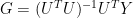
Commentary: Mann uses SVD to carry out matrix inversions. There is an identity relating the pseudoinverse used in regression calculations to Mann’s SVD methods, that is very useful in analyzing this code. If the SVD of a matrix is represented as , the pseudoinverse of X can be represented by the following:

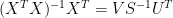
This can be seen merely by substituting in the pseudoinverse and cancelling.

Note that U,S and V as used here are merely local SVD decompositions and do not pertain to the “global” uses of U, S and V in the article, which I’ve reserved the products of the original SVD decomposition of the gridcell temperature network :

Defining L as the k=ipc truncated and normalized eigenvalue matrix and keeping in mind that is the network of retained temperature PCs, we can collect the above pseudocode as:

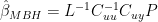
Applying the pseudoinverse identity to in the above expression, we can convert this to more familiar nomenclature:

In our emulations in 2005 (and also in the Wahl and Ammann 2007 emulation which I reconciled to ours almost immediately in May 2005), the matrix of calibration coefficients was calculated without weighting the target PCs and without weighting the proxies (in this step) as follows:

The two coefficient matrices are connected easily as follows:

The two weights have quite different effects in the calculation. The weights are ultimately cancelled out in a later re-scaling operation, but the weights carry forward and can have a substantial impact on downstream results (e.g. the NOAMER PC controversies.)

Following what seemed to be the most implausible interpretation of the sketchy description, we weighted the proxies in the estimation step; Wahl and Ammann dispensed with this procedure altogether, arguing that the reconstruction was “robust” to an “important” methodological “simplification” – the deletion of any attempt at weighting proxies (a point which disregards the issue of whether such weighting for geographical distribution or over-representation of one type or site has a logical purpose.)

Reconstruction

Scrolling down a bit further, one finds the reconstruction step in the code described as:

“DETERMINE THE RECONSTRUCTED FIELDS BY INVERTING THE TRANSFER FUNCTION”

Once again, here is a transliteration of the Fortran blizzard into matrix notation first following the native nomenclature of the code:

B0 = aprox * diag(weightprx)
#this repeats previous calculation: aprox is the proxy matrix, weightprx the weights
AA< -beta
# beta is carried forward from prior step
[UU,SS,VV] -svd(t(AA))
# again the regression is done by SVD, this time on the matrix of calibration coefficients
work0<- B0 * UU * diag( 1/SS)
work0 <-work0 * t(VV)
#this is regression carried out using the SVD equivalent to pseudoinverse
x0<- work0
#this is the matrix of reconstructed RPCs

Summarizing by collecting the terms:

[UU,SS,VV] = svd(beta) )
x0= aprox * diag(weightprx) * UU* diag( 1/SS) * t(VV)

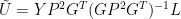
Commentary: Using our notation, the unrescaled reconstructed RPCs denoted by instead of x0 are obtained:

Once again the pseudoinverse identity can be applied, this time for where yielding:

where

Expressed in terms of C matrices, this expression becomes:

The form of the above expression is precisely identical to the form of the expression resulting from application of the conventional expression for weighted regression shown above, which was (additionally incorporating the L weighting, which is removed in a later step):

However, there is one obvious difference. The Mannian implementation, which, rather than using any form of conventional regression software, using his ad hoc “proprietary” code, ends up with the proxy weights being squared.

In a follow-up post, I’ll show how the L weighting (but not the P weighting) falls out in re-scaling.

The Wahl and Ammann implementation omitted the weighting of proxies – something that they proclaimed as a “simplification of the method”. If you have highly uneven geographic distribution, it doesn’t seem like a bad idea to allow for that through some sort of stratification. For example, the MBH AD1400 network has 4 separate series from Quelccaya glacier (out of only 22 in the regression network) – the AD!000 network has all f in a network of only 14 proxies. These consist of dO18 values and accumulation values from 2 different cores. It doesn’t make any sense to think that all 4 proxies are separately recording information relevant to the reconstruction of multiple “climate fields” – so the averaging or weighting of series from the same site seems a prerequisite. Otherwise, why not have ring width measurements from individual trees? Some sort of averaging is implicitly done already. In another case, the AD1400 network has two ring width series from two nearby French sites and two nearby Morocco sites, which might easily have been averaged or even weighted through a PC network, as opposed to being used separately.

While some methodological interest attaches to these steps, in terms of actual impact on MBH, the only thing that “matters” is the weight on the bristlecones – one can upweight or downweight the various “other” series, but the MBH network is functionally equivalent to bristlecones +white noise, so upweighting or downweighting the white noise series doesn’t really “matter”