More Mystery at Sheep Mountain

The Sheep Mountain CA bristlecone site is the most important proxy in MBH and the MBH98 reconstruction actually doesn’t differ very much from the Sheep Mountain tree ring chronology (other than it ends in 1980 at pretty much the peak of the Sheep Mt chronology and doesn’t include the downtick in the 1980s.) Various efforts by Mann and his associates to show that they can “get” a HS using various salvage methods do little more than present the bristlecone ring width chronologies up to 1980 in various wigs (borrowing Hu McCulloch’s apt phrase).

A few months ago, I reported that Linah Ababneh’s thesis contained an updated Sheep Mountain chronology which cast the matter in a provocative new light – in which even MBH wigs were of no avail. Here is the comparison that I posted up at the time showing the remarkable “divergence” between the updated Ababneh chronology and the Graybill chronology used in MBH98 (and other studies as well either directly or via the Mann PC1: Crowley and Lowery 2000; IPCC 2001; Mann and Jones 2003; Osborn and Briffa 2006; Hegerl et al 2006; Rutherford et al 2005; Mann et al 2007; IPCC 2007.) Obviously the distinctive HS shape of the Graybill chronology is not replicated in the recent Ababneh chronology. You can view a version of the original Ababneh graphic in this post
if you wish to verify that my plot here (from Hans Erren’s digitization) correctly implements the Ababneh version in her thesis.


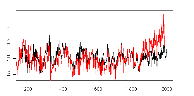
Figure 1. Ababneh and Graybill chronologies. Ababneh-black; Graybill -red.

I was doing some calculations to show the Divergence Problem in relation to these chronologies and did a short-segment Mannian standardization of these two series (on the period 1902-1980), yielding the following interesting result. In this perspective, instead of diverging in the period from 1850 on, the two chronologies match rather closely! Despite the seemingly different appearance of post-1840 values in the first plot, they are very similar after 1840 if re-scaled.

abanne48.gif
Figure 2. Ababneh and Graybill Sheep Mt chronologies, standardized on 1902-1980.

So we have a real puzzle? In Figure 1, the Ababneh and Graybill chronologies track each other closely up to about 1840. In Figure 2 (after re-scaling), the Ababneh and Graybill chronologies track each other closely after 1840. Here’s what happens: after 1840, the Graybill chronology is dilated about 186% relative to the Ababneh chronology. It’s almost a linear transformation!

This is really weird, even for dendro. What explains it? I can really only guess. However, it is surely unacceptable in any professional science to have unexplained differences like this – especially in an important series in MBH98 (and one which is even illustrated in IPCC AR4 – based on the Graybill version, of course).

We can eliminate one “explanation” pretty easily: it isn’t CO2 fertilization, since we’re talking ring width measurements at the same site presumably with many of the same trees.

One possibility is that Ababneh screwed up her chronology calculations. This seems unlikely as these calculations are pretty much canned calculations given the measurement data. These results were presented as the major part of her PhD thesis and in a recent “peer reviewed” journal article. Did anyone on her thesis committee at the University of Arizona (including Malcolm Hughes) check her calculations? While one doesn’t expect mistakes to be made with canned programs, things happen. Checking would only take about 20 minutes to do given the measurement data. Or maybe calculations aren’t checked in University of Arizona PhD theses. In her thesis, she says that she will archive her data at ITRDB, but nothing has been archived so far. I guess the dendros didn’t check that either. The University of Arizona claims not to have the data.

I have no reason to believe that her calculations are incorrect, but that leaves the dilation relative to the Graybill chronology unexplained. Should the thesis committee have asked for this to be explained in her thesis? This occurred to me immediately. Malcolm Hughes knows the Sheep Mountain chronology – it was an issue in our MBH criticisms. Why didn’t he ask that she deal with this. But, hey, it’s climate science.

The most likely difference is due to populations. Ababneh used 100 trees in her calculation – which is larger sample than that which Graybill archived. Maybe the Graybill sample was not representative. At Almagre, we found that Graybill did not archive all of the measured trees – only a subset. Nobody ever mentioned this in any literature. Is the Graybill chronology based on a specially tailored subset? This is possible: Graybill was looking for data to support his theory of CO2 fertilization and in Graybill and Idso 1993, he said that they selected strip bark trees. Maybe this explains the difference. Or maybe the Graybill sample was simply too small. Who knows? There’s no proper data archiving, no proper analysis. It’s a typical MBH mess.

What we do know is that we have inconsistent versions of the Sheep Mountain chronology – versions that are different on the key issue of medieval-modern relationships. In the Graybill version (as applied by Mann), the California “sweet spot” had bitter cold in the MWP; for whatever reason, Ababneh didn’t replicate this result.

Until the University of Arizona provides a proper explanation of the present fiasco in their Sheep Mountain records, I do not believe that any of these chronologies can be validly used in a temperature reconstruction. End of story. All calculations using Graybill’s Sheep Mountain (and Campito Mountain etc.) chronologies should be frozen and put on the sidelines until the matter is resolved – just the way a professional organization would do it.

Sure Mann can claim till he’s blue in the face that he can “get” a HS from Graybill chronologies and the rest of the MBH network using RegEM or whatever, but, as Mann himself observed some time ago, “Garbage In, Garbage Out”. If the Graybill chronologies are garbage – and until the difference with Ababneh chronologies is resolved and the Graybill chronologies validated, they must be treated as though they were garbage – MBH98, (Rutherford et al 2005, Mann et al 2007, etc.) calculations using Graybill chronologies are also unusable. Or to use Mann’s term, “garbage”.

UPDATE: Here’s an interesting figure which shows the Ababneh reconstruction scaled to match the Graybill reconstruction in the Mannian calibraiton period of 1902-1980, which vividly illustrates an interesting statistical point that I discussed in connection with Juckes – that you can have reconstructions that are virtually indistinguishable in their calibration and “verification” results with very different trajectories off in the earlier portion of the reconstruction, asking how can you objectively say that one is “right” and another “wrong”.

Here’s the Ababneh chronology rescaled to match the Graybill chronology in its recent history (I’ve used the early portion of the Graybill chronology to provide the “extension” to the Ababneh chronology.) As in Figure 2 (which is identical to Figure 3 in the latter portion), the Ababneh and Graybill chronologies are indistinguishable in terms of calibration (1902-1980) period appearance. But they are also virtually identical in the “verification period” back to 1850 – the divergence between the two series occurs either before 1840 (with Ababneh having a greater proportion of thick ring widths in the early history) or after 1840 (with Ababneh having a greater proportion of thin ring widths in the later history) – or some processing difference. Regardless of which chronology is “right”, for the multiproxy statistician – who is constrained by the “peer reviewed” time series squiggles emanating from the University of Arizona – there is no objective way of picking one version rather than the other.

abanne49.gif

Svalgaard #3

Thanks to Leif Svalgaard for his continuing support of Svalgaard discussion, which is continued here (preceded by #2 here) and #1 here.

Continued here.

Did IPCC Review Editor Mitchell Do His Job?

David Holland’s FOI request for the Review Comments on IPCC AR4 Chapter 6 (Paleoclimate) has been successful, leading to David obtaining the comments, such as they are, which have now been placed online at CA here (though not yet at IPCC.)

David Holland’s request was noted up here; last year, we noted the appalling response by IPCC lead authors to, among other things, the deletion of post-1960 Briffa reconstruction results – see for example here here here, where the lead author (Briffa) justified the deletion of adverse post-1960 results from his reconstruction merely by saying that it would be “inappropriate” to show it.

As a reviewer, I had strongly objected to the mischaracterization of the results of McIntyre and McKitrick [2003,2005a,2005b, 2005c, 2005d], as did Ross McKitrick and the Review Comments, in my opinion, dealt with our objections inadequately. In my comments as a reviewer, I distinguished between whether they correctly characterized what we said (which is a minimum expectation) and whether they endorsed our criticisms. I took particular exception to mischaracterization.

IPCC Procedures state categorically that “different (possibly controversial)” views should be described:

It is important that Reports describe different (possibly controversial) scientific, technical, and socio-economic views on a subject, particularly if they are relevant to the policy debate.

Where controversies such as this exist, Review Editors have an important role set out in IPCC Procedures as follows:

Function: Review Editors will assist the Working Group/Task Force Bureaux in identifying reviewers for the expert review process, ensure that all substantive expert and government review comments are afforded appropriate consideration, advise lead authors on how to handle contentious/controversial issues and ensure genuine controversies are reflected adequately in the text of the Report.

Comment: There will be one or two Review Editors per chapter (including their executive summaries) and per technical summary. In order to carry out these tasks, Review Editors will need to have a broad understanding of the wider scientific and technical issues being addressed. The workload will be particularly heavy during the final stages of the Report preparation. This includes attending those meetings where writing teams are considering the results of the two review rounds. Review Editors are not actively engaged in drafting Reports and cannot serve as reviewers of those chapters of which they are Authors. Review Editors can be members of a Working Group/Task Force Bureau or outside experts agreed by the Working Group/Task Force Bureau.

Although responsibility for the final text remains with the Lead Authors, Review Editors will need to ensure that where significant differences of opinion on scientific issues remain, such differences are described in an annex to the Report. Review Editors must submit a written report to the Working Group Sessions or the Panel and where appropriate, will be requested to attend Sessions of the Working Group and of the IPCC to communicate their findings from the review process and to assist in finalising the Summary for Policymakers, Overview Chapters of Methodology Reports and Synthesis Reports. The names of all Review Editors will be acknowledged in the Reports.

John Mitchell, Chief Scientist, UK Met Office is an experienced administrator. The entire text of his Review Editor Comments (as disclosed by FOI) are as follows:

As Review Editor of Chapter 6, …I can confirm that the authors have in my view dealt with reviewers’ comments to the extent that can reasonably be expected. There will inevitably remain some disagreement on how they have dealt with reconstructions of the last 1000 years and there is further work to be done here in the future, but in my judgment, the authors have made a reasonable assessment of the evidence they have to hand. The other possible area of contention(within the author team) is on some aspects of sea-level rise. This has gone some way towards reconciliation but I sense not everyone is entirely happy.

With these caveats I am happy to sign off the chapter …

Mitchell’s sign-off letter explicitly recognized that there was “some disagreement on how they have dealt with reconstructions of the last 1000 years”. In such circumstances, is it enough for him to simply arrive at a personal judgment that
“in his judgment, the authors have made a reasonable assessment of the evidence they have to hand”. I don’t think so. One assumes that IPCC authors will make a “reasonable” assessment; that’s not the issue for Mitchell in his capacity as a Review Editor. His obligation was to ensure that the Report described “different (possibly controversial) scientific views” on the 1000-year reconstructions and to ensure “where significant differences of opinion on scientific issues remain, such differences are described in an annex to the Report”. Did Mitchell do this? Sure doesn’t look like it to me.

In addition, I must say that I’m surprised at how perfunctory Mitchell’s letter was. This must have taken him all of 30 seconds to write.

The covering letter from the IPCC WG1 TSU to David Holland stated:

Dear Dr Holland,

Thank you for your interest in the Working Group I contribution to the IPCC Fourth Assessment Report.

Please find attached a copy of the Review Editor Report from Dr John Mitchell on Chapter 6 Paleoclimate of the Working Group I contribution to the IPCC Fourth Assessment Report, “Climate Change 2007: The Physical Science Basis”.

Best regards,
Melinda Tignor
WGI TSU

Perhaps Mitchell made other comments and IPCC and the UK FOI have failed to provide these other comments. It would probably be worthwhile renewing the request under the UK FOI legislation to ensure that there really is nothing else. It’s not like IPCC to be fulsome in their responses. On the basis of the correspondence provided by IPCC, Mitchell’s contribution as Chapter 6 Review Editor are so minimal that he’s rendered the office of Chapter 6 Review Editor pretty much useless. One surely would expect more from a senior U.K. scientist and experienced scientific administrator.

If this is all that Mitchell contributed, the quality of the comments by the Chapter 6 Review Editor hardly support claims that the IPCC review process is some sort of model review process. In saying this, I’m not saying that the fact that Mitchell made perfunctory comments as Review Editor proves that anything in the report is wrong; the report is written by experienced and knowledgeable scientists and, as such, warrants careful consideration. However, in the corner of the IPCC report with which I’m most familiar – the 1000 year reconstructions – Review Editor Mitchell did not discharge all his IPCC responsibilities and acquiesced in a section that contained a rather one-sided exposition of a relevant controversy and the lamentable quality of his Comments show his acquiescence in this particular section of the IPCC Report failing to meet IPCC standards.

Update:
David Holland reports that “WGI TSU have just sent me Dr Jouzel’s report”. Here is his transcription:

As Review Editor of Chapter 6 Paleoclimate of the Working Group I contribution to the IPCC Fourth Assessment Report, “Climate Change 2007: The Physical Science Basis”, I can confirm that all substantive expert and government review comments have been afforded appropriate consideration by the writing team in accordance with IPCC procedures.

Hansen and Hot Summers in the Southeast

Hansen et al 1988 reported that they expected extra warming in the SE United States, a theme that was mentioned in his testimony in Washington in summer 1987. Hansen et al 1988 stated:

there is a tendency in the model for greater than average warming in the southeastern and central U.S. and relatively cooler or less than average warming in the western U.S. and much of Europe in the late 1980s and in the 1990s. …

We also notice a tendency for certain patterns in the warming, for example, greater than average warming in the eastern United States and less warming in the western United States. Examination of the changes in sea level pressure and atmospheric winds suggests that this pattern in the model may be related to the ocean’s response time; the Atlantic off the Eastern U.S. and in the Pacific off California tends to increase sea level pressure in those ocean regions and this in turn tends to cause more southerly winds in the eastern U.S. and more northerly winds in the western U.S. …

Monthly temperature anomalies can be readily noticed by the average person or ‘man in the street’. A calibration of the magnitude of mode predicted warming can be obtained by comparison of Plate 6 with maps of observations for recent years as published by Hansen et al 1987 using the same color scale as employed here. This comparison shows that the warm events predicted to occur by the 2010s and 2020s are much more severe than those of recent experience such as the July 1986 heat wave in the southern U.S., judging by the area and magnitude of the hot regions.

Here is a an excerpt from Hansen et al Plate 2 illustrating the model output which supported this observation. Scenario B is the one that corresponds more closely to actual forcing. I’ve shown Scenario as well, on the basis that Scenario B is only shown here for the 1990s and arguably Scenario A in the 1990s yields insight into Scenario B in the 2000s. The salient point of the diagram here is the structure of the “dipole” clearly visible in A in which there is cooling in the western US and warming in the eastern US. In Scenario B, the dipole is less evident, but is perhaps directionally there as well.

southe3.jpg

There are many interesting aspects to this. Remember Michael Mann’s claim in regard to bristlecone pines – that the southwestern U.S. is a “sweet spot” for measuring climate change. In Hansen’s model, the southwest U.S. has very anomalous behavior. For some reason, in Scenario A in the 1990s, it is one of only a couple of regions in the entire world where Hansen’s model predicted cooling. Seems like an odd sort of “sweet spot” for measuring global temperature.

Now here are several plots showing observed trends. First here is a plot that I did earlier based on USHCN TOBS data (annual here rather than summer – I’ll try to do summer as well some time, but this is what I have on hand). Again one sees sort of a “dipole” structure between the eastern and western US that resembles the dipole structure in the Hansen et al 1988 model with one small problem – the sign of the change is reversed.

southe4.gif

For someone that’s worried about whether my calculations of 20th century trends are accurate, here is a figure from AR4 also showing a cooling trend in the southeast and a warming trend in the west.
southe12.jpg

Actually AR4 even has a map that supports the point for JJA temperatures from 1979-2005, as shown in the graphic below:

southe13.jpg

I also did a quick calculation making an annual and JJA average for all USHCN stations (TOBS) that were located east of 100W and south of 37N as a rough approximation to the southeast. Here’s the result that I got. Based on this calculation, the number of warm summers in the period 1987-2007 is greater than the period 1951-80 (“climatology” in Hansen et al 1988) but not greater than the period 1920-1940 for example.

southe5.gif
Average calculated for USHCN stations east of 100W; south of 37N ; red is 1987

Again I’m not saying that any of these details disprove GHG forcing. However Hansen specifically discussed the southeast US both in his article and emphasized it in his testimony and the actual results should be at least canvassed briefly before saying that Hansen is the new Nostradamus.

It’s also interesting to contrast the presentation of this topic in Hansen et al 1988 with Hansen’s 1988 testimony here. The description of warming in the eastern U.S. in the testimony tracked the corresponding text in the original article quite closely as you can see in the excerpt below:

in the late 1980s and in the 1990s, we notice a clear tendency in the model for greater than average warming in the southeast U.S. and the midwest….In our model this result seems to arise because the Atlantic Ocean off the coast of the U.S. warms more slowly than the land. This leads to high pressure along the east coast and circulation of warm air north into the midwest or the southeast. There is only a tendency for this phenomenon. It is certainly not going to happen every year and climate models are certainly an imperfect tool at this time. However we conclude that the greenhouse effect increases the likelihood of heat wave drought situations in the southeast and midwest U.S. even though we cannot blame a specific drought on the greenhouse effect.

But there is one noticeable difference between his 1988 testimony about what the model predicted for the United States and what was mentioned in the corresponding text in Hansen et al 1988. See if you can find it.

Hansen in Antarctica

Hansen et al 1988 noted very sensibly that there were radically different approaches to some physical problems in GCMs and looked forward to the “real world laboratory in the 1990s” providing empirical information on these conundrums. One such conundrum were temperatures offshore Antarctica. They noted that their model showed a strong warming trend in sea ice regions bordering Antarctica while Manabe’s model showed cooling after CO2 doubling, a difference hypothesized to arise from differing ocean heat transport assumptions.

This was a fairly posed observation and I thought it would be interesting to see how things turned out in the next 20 years, not, as criticism of the 1988 model, but merely to see whether subsequent information shed any light on these questions. In an earlier post, we inquired about Waldo in Antarctica . Today his cousin Hansen.

First here is an excerpt from Plate 2 from Hansen et al 1988 (lowball Scenario C not being shown in this excerpt) showing the decadal mean temperature increase relative to the control run mean for Scenarios A and B in the 1990s for DCF and JJA. The forcing history has been closer to Scenario B than to Scenario A; but, in the absence of such a graphic in Hansen et al 1998 showing the 2000s, perhaps Scenario A in the 1990s can be interpreted as an rough approximation to Scenario B in the 2000s. (I’m not placing any weight on this interpretation here, merely noting it to guide your eye.) I want you to look today at the offshore Antarctica area, where Hansen expressed uncertainty about his physical parameterizations. We can talk about other areas on other occasions.

southe10.jpg
southe14.jpg

For comparison, here is an IPCC AR4 figure showing 1979-2005 tropospheric trends. This is an annual basis, while the Hansen figure shows two seasons. So you’ll have to “add up” the colors in the Hansen figure to compare. But, for a qualitatitive impression, it’s easy enough to do. John Christy pointed out yesterday that you need to multiply troposphere trends by 1.2 to match surface trends so keep that in mind – though the discussion here is only of patterns. There’s not much texture in the DJF offshore Antarctica in the 1990s, so most of the texture comes from the JJA period shown in the left bottom Hansen figure above; these changes would be attenuated when an annual average is taken.

southe11.jpg

I’d like you to look at the pattern of increase and decrease around Antarctica in each figure. In the real world, there is a a cooling area off Antarctica to the south of Africa, a warming area to the southwest of Australia and another cooling area on the bottom right of the graphic reaching up towards New Zealand.

Now compare this to Scenario B in the 1990s. As noted above, most Scenario B texture offshore Antarctica occurs in the SH winter (JJA), where we see almost the reverse pattern to the one predicted in Hansen et al 1988. Off to the bottom right of the Hansen figure (bottom left panel) we see strong warming predicted in the area SW of New Zealand where cooling occurred in the real world; we see cooling predicted in the area to the SW of Australia where warming occurred in the real world and we see strong warming predicted south of Africa, where cooling occurred. At the Antarctic Peninsula, Hansen predicted negligible change in summer (DJF) temperatures. In the area south of the Atlantic just to the east of South America, both model and result were warm.

What struck me here was the “remarkable similarity” in the geometric pattern between the model and the outcome, with lobes southwest of New Zealand, southwest of Australia and south of Africa nicely matching. The only defect from a modeling point of view was that these predictions offshore Antarctica had the wrong sign. So to the extent that Hansen was wondering about his Antarctic sea ice model in 1988, it looks like some wrong choices were made for this particular aspect of his model. It would be an interesting inquiry to track how the GISS sea-ice module was modified in subsequent versions as to the sea-ice module.

I note that there is also a problem in sea-ice formation in the more recent ECHO-G model which I noticed in their data, but haven’t discussed previously.

I am not suggesting that a mis-step in modeling Antarctic sea ice in Hansen et al 1988 (especially where uncertainty was noted at the time) invalidates other aspects of his predictions. However as to Hansen’s predictions for offshore Antarctica, I would certainly not regard them as “eerily” prescient and indicate the need for a little caution in other parts of the package to understand better what aspects have stood the test of time and what haven’t.

One of the retorts to observing any inaccuracy in a model always seems to be – well, the error doesn’t “matter”, we get the same answer anyway. My instinct from mathematics is then: well, if you get the same answer for doubled CO2 both ways, surely there is some sort of relevant simplification that would assist in laying bare the mechanics of the GCM in question. My instinct in all of this is that the GCMs are an interesting intellectual exercise, but a needless complication of the relevant physics for developing policy on doubled CO2. I’m not asserting this ex cathedra; it’s merely my instinct at this time.

Hansen 1988: Details of Forcing Projections

During our discussions of the differences between Hansen Scenarios A and B – during which the role of CFCs in Scenario A gradually became clearer – the absence of a graph clearly showing the allocation of radiative forcing between GHGs stood out rather starkly to me. When Gavin Schmidt re-visited the topic in May 2007, he only showed total forcing both in his graphic here (see below)and in the data set http://www.realclimate.org/data/H88_scenarios_eff.dat .


Figure 1. Forcing totals form Schmidt (2007)

Schmidt summarized the differences as follows:

The details varied for each scenario, but the net effect of all the changes was that Scenario A assumed exponential growth in forcings, Scenario B was roughly a linear increase in forcings, and Scenario C was similar to B, but had close to constant forcings from 2000 onwards. Scenario B and C had an ‘El Chichon’ sized volcanic eruption in 1995.

While it is true that the total forcing in Scenario A is “exponential” and the forcing in Scenario B is “linear”, the graphic below shows my estimates of how the forcing breaks down between GHGs within each of the three scenarios using contemporary or near-contemporary “simplified expressions”.

forcin86.gif
Figure 2. Radiative forcing for three Hansen scenarios and calculations based on observed and A1B GHG concentrations.

Obviously one point sticks out like a sore thumb: Scenario A increases are dominated by CFC greenhouse effect. In Scenario A, the CFC contribution to the Earth’s greenhouse effect becomes nearly double the CO2 contribution during the projection period. This is not mentioned either in Hansen et al 1988 or in Schmidt (realclimate, 2007).

The allocation between GHGs also clarifies why Scenario B is “linear” and Scenario A “exponential”. In Scenario B, the main forcing occurs from CO2 increase (not CFC increase). The “simplified expression” for the relationship between CO2 concentration and temperature change is logarithmic; thus, even though CO2 growth is (modestly) exponential in Scenario B, the composite of the exponential increase in GHC concentration and a logarithmic expression relating CO2 concentration to forcing yields linear growth in forcing.

On the other hand, the simplified expression relating CFC concentration to forcing is linear. Thus the exponential growth in CFC concentration in Scenario A (and the CFC growth rate is hypothesized to be much stronger than for CO2), combined with a linear relationship leads to an exponential growth in total forcing – driven primarily by CFCs.

Calculation Method
The GHG concentrations used for the above calculations are taken from the file posted at realclimate on Dec 22, 2007 ( http://www.realclimate.org/data/H88_scenarios.dat ). Something close to these concentrations could be calculated from the verbal descriptions of Hansen et al 1988 (as I had done here […] prior to becoming aware of this file at realclimate).

Hansen et al 1988 contained a series of “Simplified Expressions” relating forcing (in delta-T) to GHG concentrations for each of the GHGs. Usual current practice is to express forcing as wm-2; IPCC 1990 (p 52) said that a factor of 3.35 was needed to convert the Hansen equations to wm-2 and this has been applied here. (For the CFC11 and CFC12 equations, which could be checked directly, this conversion factor reconciles the Hansen expression to the IPCC 1990 expression.) I was unable to get the Hansen et al 1988 expressions for CH4 and N2O forcing to yield sensible results and for these two gases, I used the expression in IPCC 1990 to convert GHG concentration to radiative forcing. If anyone can get the Hansen et al 1988 expressions for CH4 and N2O to work, I’d be interested. I spent a fair bit of time on this before abandoning the effort and going with the IPCC 1990 expressions.

In all cases, I’ve used the “pre-industrial” concentrations used by NOAA in their calculations. In some Hansen calculations, a 1958 base is used (and these differences can be readily reconciled at least to a first approximation.)

Discussion

Hansen et al 1988 said that “resource limitations” ultimately checked the expansion of Scenario A. While this is true for CO2, I’m a bit dubous that resource limitations come into play in connection with CFC emissions. Obviously CFC emissions have not increased anywhere like Hansen Scenario A. I can’t comment on whether this is due to Montreal Protocols or other factors, but “resource limitations” seem highly unlikely as a limiting factor for CFC growth history.

Second, while Hansen et al 1988 disclosed that they doubled the CFC11 and CFC12 contributions to account for minor CFCs, this seems like a pretty aggressive accounting, especially in a context of very strong CFC11 and CFC12 growth. Without an illustration of the allocation of forcing by GHG, an innocent reader of this article could easily assume that the doubling was a simple and reasonable way to deal with a minor effect and immaterial to the results. If the assumption is material (as it is), then the treatment and analysis of this assumption seems far too casual.

Third, one wonders how much subsequent controversy might have been avoided if Hansen et al had clearly shown and discussed the allocation between GHG in the clear form shown above. Here is how Hansen et al 1988 Figure 2 showed the results:

forcin6.gif
Figure 3. Total forcing from Hansen et al 1988 Figure 2. Multiple by 3.35 (IPCC 1990) to get wm-2.

In my opinion, this graphic does not clearly show that CFC contribution to Hansen’s greenhouse effect in Scenario A becomes double that of CO2. Aside from the graphic, the running text does not clearly state that CFC greenhouse contributions exceed CO2 contributions during the projection period. Had there been a clearer graphic together with an explicit recognition of CFC contribution, people would have been able to look past Hansen’s unfortunate description of Scenario A as “Business As Usual” in his 1988 testimony and see that it was really an implausible upper bracket scenario, just as Scenario C was an implausible lower bracket scenario, and place no weight on Hansen’s “Business as Usual” label. In passing, Hansen’s 1987 testimony , not previously discussed here, provided the following further information on Hansen’s views on the respective merits of these scenarios:

Scenario A assumes that CO2 emissions will grow 1.5% per year and that CFC emission will grow 1.5% per year. Scenario B assumes constant future emissions. If populations increase, Scenario B requires emissions per capita to decrease. Scenario C has drastic cuts in emissions by the year 2000, with CFC emissions eliminated entirely and other trace gas emissions reduced to a level where they just balance their sinks. These scenarios are designed to cover a very broad range of cases. If I were forced to choose one as the most plausible, I would say Scenario B. My guess is that the world is now probably following a course that will take it somewhere between A and B. (p. 51)

If one is trying to evaluate Hansen’s skill as a forecaster of GHG concentrations, I think that this is probably the most reasonable basis – thus, some sort of weighted average of A and B, with somewhat more weight on B would seem appropriate.

Fourth, one has to distinguish between Hansen’s abilities as a forecaster of future GHG concentrations and the skill of the model, with Hansen himself obviously placing more weight on his role as modeler than as a GHG forecaster. To the extent that “somewhere between A and B” represents Hansen’s GHG forecast, in that GHG increases appear to have been closer to B than “somewhere between A and B”, it is more reasonable to use B to assess the model performance. (It would be more reasonable still for NASA to re-run the 1988 model with observed results.)

Fifth, Hansen argued vehemently that the skill of his results should not be assessed on Scenario A results. Fair enough. The difference between Scenario A and Scenario B points to the need to look carefully at GHG concentration projections in forecasts, which in 2007 are the IPCC SRES projections. The evaluation of the IPCC SRES projections becomes an important and perhaps under-appreciated activity. If one is prepared to agree with Hansen’s position that he should not be assessed on Scenario A (and I, for one, am prepared to agree on this), then it points to the need for caution in using publicizing results from today’s version of Scenario A GHG (e.g. perhaps IPCC A2), a point raised by Chip Knappenburger at RC.

Sixth, none of these calculations deal with feedbacks. So the sort of numbers that result from these calculations are in the range of 1.2 deg C for doubling CO2, depending on the precise radiative-convective model. In this case, the “simplified expressions” are based on the Lacis et al 1981 radiative-convective model and not from GCMs. Similar results are obtained with other radiative-convective models and someone seeking to dispute the results would need to show some systemic form of over-estimation in the radiative-convective models.

Seventh, Hansen et al 1998 , not cited in Schmidt (2007), contains an interesting and reasonable discussion of the 1988 scenarios ten years later and I’ll review this discussion some time in a subsequent post.

Prior discussions in posts http://www.climateaudit.org/?p=2630 and http://www.climateaudit.org/?p=2638.

NOAA training manual cites errors with Baltimore's Rooftop USHCN Station

I happened across a NOAA internal training manual a couple of weeks ago that contained a photo of a USHCN official climate station that I thought I’d never get a photo of. The Baltimore Customs House.

Baltimore Customs House USHCN
Baltimore USHCN station circa 1990’s photo courtesy NOAA, click for more images

What is interesting about this station, is that it is a rooftop station, like we’ve seen in San Francisco, Eureka, and many other US cities. Rooftop stations are suspected to impart a warm bias to the surface temperature records, for obvious reasons. The NWS/NOAA has been reluctant to change these stations to ground-level, wanting to keep a continuous record. The Baltimore USHCN station closed in 1999 and has not been replaced at this location.

Continue reading

RSS Corrects 2007 Error

On January 16, 2008, I posted a note on Hansen et al 1988 containing the following graphic comparing the three Hansen scenarios to the most recent GISS and RSS temperature versions.
.

Although there had been much furore in the past about the differences between Hansen Scenarios A and B in previous controversy, I observed that Scenarios A and B were both at very elevated levels by 2010 and that noticeable increases in RSS temperature would be required to keep pace even with Hansen Scenario B. While I expressed this in terms of the RSS data, the same thing is true for the GISS surface data.

This graphic used the following file downloaded from RSS on January 16, 2008
http://www.remss.com/pub/msu/monthly_time_series/RSS_Monthly_MSU_AMSU_Channel_TLT_Anomalies_Land_and_Ocean_v03_0.txt

Eli Rabett today accused me of using “an older version” of the RSS temperature reconstruction as follows:

But lo, our auditors had also used an older version of the RSS microwave tropospheric temperature reconstruction. It had a serious error. What does the corrected version look like?

An older version?

Two days after my post, on January 18, 2008, RSS issued an amended version of their TLT data http://www.remss.com/pub/msu/monthly_time_series/RSS_Monthly_MSU_AMSU_Channel_TLT_Anomalies_Land_and_Ocean_v03_1.txt

Unfortunately, there is no announcement of the error at the RSS homepage http://www.remss.com/msu/msu_data_description.html. As far as I know at present, the only notice of the error is through a readme (http://www.remss.com/pub/msu/data/readme_jan_2008.txt ) dated January 16, 2008, but only posted up on January 18, 2008 (see http://www.remss.com/pub/msu/data/ ) . Rabett did not state how he happened to become aware of the readme mentioning the error as to my knowledge, it is not linked through the home page or through an explicit announcement. Rabett linked to the readme, carefully including the reported date of January 16, 2008, but failing to mention that the readme was posted on Janueary 18, 2008 (also after my post).

Last January, I made a small change in the way TLT is calculated that reduced the absolute
Temperatures by 0.1K. But I only used the new method for 2007 (the error).
When the data are merged with MSU, MSU and AMSU are forced to be as close as possible to each
other over the 1999-2004 period of overlap. This caused the error to show up as a downward
jump in JAnuary 2007. To fix the problem, I reprocessed the 1998-2006 AMSU data using the new
code (like I should have done in the first place), and merged it with the MSU data.

We would like to thank John Christy and Roy Spencer, who were very helpful during the diagnosis
process.

Carl Mears, RSS, January 16 2008

Thus, on January 16, 2008 when I did my post, I was using the current RSS version. Yes, two days later, RSS changed their 2007 numbers. Here are two graphics showing the impact of the RSS changes – Jan 3, 2008 (red) and Jan 18, 2008 (blue):
rssht4.gif

and a second one showing the difference between the two series, which works out to about 0.12-0.14 deg C during 2007.

rssht99.gif

Also here is a revised version of my graphic, implementing the Jan 18, 2008 RSS changes. The main point of my earlier post clearly stands — in 2010, the difference between Scenarios A and B is not particularly large and some of the past furore over scenario versions becomes less material.

rssht1.gif

In his coverage of the RSS error, Rabett disparaged my analysis, implying that, by using an “older version” of the RSS data, I had done something improper. Rabett misleadingly failed to cite the dates of the RSS versions, which would have shown that I had used the then current RSS version (Jan 3, 2008, then current as at Jan 16, 2008) and that that the newer version (Jan 18, 2008) was not available at the time of my post. Rabett shows the readme dated January 16, 2008 implying that I should have been aware of it (even though it is nowhere linked on the RSS webpage) without stating that it was posted on January 18, 2008 subsequent to my post.

In the same post that Rabett criticized here, as originally written, I had incorrectly missed a comment in Hansen et al 1988 saying that Scenario B was the “most plausible”, an error which I picked up about 8 hours after the original posting (about 9 am EST) and immediately corrected it when I noticed it. So there was an actual incorrect statement at CA for about 8 hours. Imagine that. I didn’t post up notice of the change until about 9 hours later (I was playing in a squash tournament and had to do some chores and went out after making the correction and posted the notice when I returned.) Meanwhile, a few hours after I made the correction, Lambert wrote a post on this error without mentioning that the error had already been corrected as at the time of his post. This caused a tizzy of excitement over at Deltoid over the possibility that I might actually have made a mistake on something (outside my core area). Gavin Schmidt interrupted his day at NASA to weigh on the matter at Deltoid.

I don’t claim to be infallible. I corrected this particular error promptly. Compare the treatment of an error in an incidental blog post that I corrected within about 8 hours to the treatment of the RSS error. Do Rabett or Lambert excoriate RSS for their goof? A goof that occurred in a high-profile data set? Of course not. To the extent that they place any blame, Rabett blames me for not using an RSS version that didn’t even exist at the time of the post.

As to RSS, they made a mistake and corrected it. Good for them. Errors happen and RSS corrected their error. Rabett observed of the RSS error:

PPS: Lots of folk are falling into the RSS error trap.

Rabett proceeds to blame users of RSS data. The fact that users are “falling into the RSS error trap” is one more good reason why RSS should have issued a clear error notice, rather than the obscure readme. They should issue a proper notice of the error in their public webpages and wherever else appropriate. They were pretty quick to publicize errors by Spencer and Christy and should accord equal publicity to their own error.

Update Jan 24, 2008 12.40 pm:

Here is a version showing including the MSU version centered to synchronize with GISS for the period up to 1987. As you can see, the MSU version was bracketed by the GISS and old RSS versions. These spaghetti graphcs get pretty messy pretty fast and since it was bracketed, I did not include it in my prior version. Eli Rabett has made an issue of this and I have accordingly shown the MSU version here on the same basis as the prior graphic. As you see, it is no longer bracketed by GISS and the new RSS version, but is slightly lower than either, the point of my post remaining unaffected.

rssht5.gif

Update: Jan 27, 2008
John Christy observed below that “one must either multiply the surface by 1.2 or divide the troposphere by 1.2” to gave apples and apples. I will re-plot the graphic once I clarify a point on this.

Loehle Correction

Craig Loehle has responded to various criticisms and issued a correction here, which he asked me to note. He states that:

the original and correction are pasted together. It has data, urls, a map, proper confidence intervals and hypothesis tests, and corrections to dating issues Gavin found

He states that “the shape of the curve didn’t change appreciably.”

In contrast, Mann et al 2007 continued to use incorrect locations for their precipitation series (the rain in Maine still continues to fall mainly in the Seine, while the rain in Bombay still continues to cause rainouts for the Phillies), and he continues to use his incorrectly calculated PC series.

It is remarkable to compare the alertness of the climate science community in this instance to the somnolent reviewing at the Journal of Climate for Mann et al 2007 – where the reviewers either didn’t bother checking whether Mann had fixed known errors or didn’t care. It is encouraging that Loehle responded promptly to the criticism by issuing a correction.

I am only posting a notice of the correction at this time, as I have not yet parsed through the details.

Radiative Forcing #1

Update: see further discussion here

NOAA has a webpage on radiative forcing here, which includes a list of equations relating GHG concentrations to radiative forcing, substantially identical to the expressions in TAR.

Below is a figure showing, on the left, the graphic at NOAA illustrating their calculation and, on the right, my emulation of this graphic from original GHG concentration data using the radiative forcing equations summarized at NOAA – so I’ve obviously got this calculation down pretty well. My text for generating this graphic is online here http://data.climateaudit.org/scripts/forcing/forcing.noaa_graphic.txt.

 hansen36.jpg  forcin76.gif

The calculation uses my collation of GISS GHG concentration data which I’ve posted up at http://data.climateaudit.org/data/hansen/giss_ghg.2007.dat . I’ve done my own collation because the GISS information is maintained (messily) in several different files:
1850-2000 from http://data.giss.nasa.gov/modelforce/ghgases/GHGs.1850-2000.txt
2001-2004 from http://data.giss.nasa.gov/modelforce/ghgases/GHGs.Obsv.2001-2004.txt
2005-2006 from individual files for each gas, estimating 2005-2006 for two trace gases where data not shown

The function to calculate forcing provides for implementing different sets of equations, not all of which are tested yet.

Whlie NOAA implementation was straightforward, this is not the case for Hansen et al 1988 and other articles. Sometimes the problems are units: Hansen et al 1988 Appendix B expressed forcing in terms of global temperature change and not in terms of wm-2. Unlike the original article, Gavin Schmidt’s Hansen et al 1988 scenario data is expressed in wm-2 (a unit not yielded by the equations of the original article.) IPCC 1990 discusses the conversion to wm-2 as follows (p 52):

“Values derived from Hansen et al have been multiplied by 3.35 (Lacis, pers comm) to convert forcing as a temperature change to forcing as a change in net flux at the tropopaus after allowing for stratospheric temperature change. These expressions should be considered as global mean forcings; they implicitly include the radiative effects of global mean cloud cover.

Using this conversion, the equations for CFC11 and CFC12 immediately translate. However, the translation for other equations is not as easy.

IPCC 1990 Table 2.2 says that, fr CO2, CH4 and N2O, they say that the “functional form [was derived] from Wigley 1987; coefficient derived from Hansen et al 1988”. I can confirm the functional form from Wigley 1987, but Hansen et al 1988 set out coefficients for different functional forms. I’ve been unable to locate any of the IPCC 1990 coefficients in original articles – I wonder where they came from.

The same problem occurs for the overlap equation for CH$ and N2O in IPCC 1990. Although the overlap term is attributed to Hansen et al 1988, the expression in IPCC Table 2.2 does not occur in either Hansen et al 1988 or Wigley 1987 – where did it come from?

I can get the IPCC 1990 overlap expression to yield sensible values, but I can’t get the Hansen et al 1988 expression to yield sensible values so far – if anybody else can, I’d appreciate the info. IPCC 1990 also mentions (also on p 52) a typographical error in Hansen et al 1988 (“0.014 should be 0.14”).

In summer 2007, Gavin Schmidt reported the GHG concentrations for the three Hansen 1988 scenarios at and the total radiative forcing (wm-2) for the three Hansen scenarios here .

I’m hoping that I will be able to replicate the Hansen radiative forcing total (at RC here http://www.realclimate.org/data/H88_scenarios_eff.dat) from the GHG concentration data (http://www.realclimate.org/data/H88_scenarios.dat) using contemporary equations and then compare this to the observed radiative forcing. In passing, I note that the structural links between Hansen et al 1988 and IPCC 1990 are quite close and provide some mutual clarification.

Also see – http://data.giss.nasa.gov/modelforce/ghgases/