I’ve posted in the past on the mystery of MBH confidence interval calculations, especially the mysterious MBH99 confidence intervals (another Caramilk secret). In our NAS panel presentation and perhaps before, I’d speculated that MBH98 confidence intervals, rotundly described in MBH98 as “self-consistently estimated”, were nothing other than twice the standard error of the (overfitted) calibration period. (May 3, 2006: Eduardo Zorita supports this interpretation in comment below.) Reader Jean S, a post-doc in statistics, has sent in a very pretty proof of this.
Based on this proof and a couple of other comments from Jean S, we’ve corresponded back and forth on the MBH99 confidence interval mystery and have reduced the mystery to a few elements, where we invite new ideas.
Review
I made two posts on the topic last May here and here . Confidence intervals are described in MBH98 as follows:
The reconstructions have been demonstrated to be unbiased back in time, as the uncalibrated variance during the 20th century calibration period was shown to be consistent with a normal distribution (Figure 5) and with a white noise spectrum. Unbiased self-consistent estimates of the uncertainties in the reconstructions were consequently available based on the residual variance uncalibrated by increasingly sparse multiproxy networks back in time [this was shown to hold up for reconstructions back to about 1600.”
….
The histograms of calibration residuals were examined for possible heteroscedasticity, but were found to pass a x2 test for gaussian characteristics at reasonably high levels of significance (NH, 95% level; NINO3, 99% level). The spectra of the calibration residuals for these quantities were, furthermore, found to be approximately ‘white’, showing little evidence for preferred or deficiently resolved timescales in the calibration process.” Having established reasonably unbiased calibration residuals, we were able to calculate uncertainties in the reconstructions by assuming that the unresolved variance is gaussian distributed over time. This variance increases back in time (the increasingly sparse multiproxy network calibrates smaller fractions of variance), yielding error bars which expand back in time.
MBH98 Figure 5 didn’t actually show that “uncalibrated variance during the 20th century calibration period was shown to be consistent with a normal distribution”. It simply showed a muddy version of the MBH98 reconstruction together with (supposed) two-sigma confidence intervals.

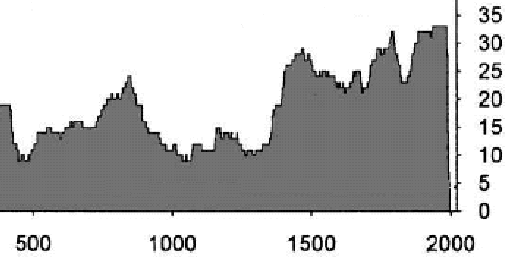
Figure 1. MBH98 Figure 5b. Original Caption: For b raw data are shown up to 1995 and positive and negative 2j uncertainty limits are shown by the light dotted lines surrounding the solid reconstruction, calculated as described in the Methods section
MBH99 said:
In contrast to MBH98 where uncertainties were self-consistently estimated based on the observation of Gaussian residuals, we here take account of the spectrum of unresolved variance, separately treating unresolved components of variance in the secular (longer than the 79 year calibration interval in this case) and higher-frequency bands. To be conservative, we take into account the slight, though statistically insignificant inflation of unresolved secular variance for the post-AD 1600 reconstructions. This procedure yields composite uncertainties that are moderately larger than those estimated by MBH98, though none of the primary conclusions therein are altered.
Poor Jean S almost gagged on Mannian prose. (Interestingly, when the MBH99 “correction” to the confidence intervals was done, Mann did not notify Nature and issue a corrigendum at Nature. In fact, if you go to the 2004 Corrigendum, you will see that the MBH98 confidence intervals are re-iterated even though they were supposedly re-calculated in MBH99).
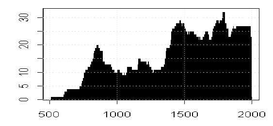
Last year, I showed the difference between the estimates in the two attempts in the following graphic.
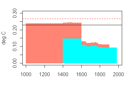
Figure 2. MBH98 and MBH99 sigma by calculation step. Cyan – MBH98; salmon – MBH99. Solid black – CRU std dev; dashed red -“sparse” instrumental std. dev.
At the time, I presumed that the difference was connected to this sentence about “separately treating unresolved components of variance in the secular (longer than the 79 year calibration interval in this case) and higher-frequency bands.”, but was then (and still am) unable to decode the rotund and uninformative language.
I re-visited the topic in December when I noted a similar phrase in Rutherford et al 2005 and surveyed some rotund Mannian literature such as Mann and Lees. This post is a handy reference for original quotations.
We referred to confidence interval issues at length in our NAS panel presentation as follows:
Confidence intervals in MBH98 (to which the term “self-consistent” is applied) are, as we understand it, calculated simply as twice the standard error from calibration period residuals. If there is overfitting (or spurious regression) in the calibration period, as appears almost certain, then calibration period residuals are likely to provide an extremely biased and over-confident estimate of confidence intervals.
For a sui generis procedure with little knowledge of its statistical properties, at a minimum, it seems to us that confidence intervals should be calculated from the verification period residuals – a procedure which was used in Mann and Rutherford [2002]. In this case, given that the verification r2 for the early steps is ~0, this procedure would, of course, have led to very wide confidence intervals and little to no reduction from natural variability, hence a complete inability to assess the statistical significance of warmth in the 1990s.
MBH99 acknowledged that there was significant low-frequency content in the spectrum of residuals i.e. highly autocorrelated residuals. Since at least Granger and Newbold [1974], econometricians have interpreted autocorrelated residuals as evidence of a misspecification. Instead, MBH99 purported to adjust the confidence interval calculations. However, no statistical reference is provided for this calculation. Neither we nor a time series specialist who we consulted on this matter have been able to figure out how this calculation was done. The use of calibration period residuals to estimate confidence intervals is followed in other multiproxy studies. In all cases, we see evidence of spurious relationships in the calibration period with serious out-of-sample behavior, raising in every case the spectre of over-optimistic estimation of the success of the reconstruction.
Jean S. re-opened the matter by sending me the following graph (slightly redrawn here by me) showing a link between MBH98 confidence intervals in each step and the calibration r^2 statistic (described by Mann as the calibration beta statistic). Jean S estimated the calibration sigma using the archived calibration r^2 statistics using the formula:
sigma = sqrt (1- r^2 [calibration]) * var (instrumental) )
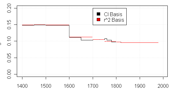
Figure 3. Comparison of observed MBH98 confidence interval to Jean S estimate. Black – from MBH98 archive; red- Jean S estimate using above formula and archived calibration R2 value. The instrumental, MBH98 reconstruction and MBH98 sigmas can be located in the following data set. Link (mirrored at WDCP and Nature). The r^2 [calibration] can be picked up here (formerly at the Nature SI, but now deleted there), where it is described as a “calibration beta” statistic.
Now I’d figured out/speculated that MBH98 confidence intervals were connected to calibration r^2 quite a while ago, but only now has Jean S figured out the exact connection. Jean S had expletives for Mannian terminology. I’ve cited a couple of his references below.
Since calibration residuals had been used by Mann in MBH98 to (1) calculate calibration r^2 and (2) 2-sigma confidence intervals, the connection between the two measures is what you expect. Since there is limited available (unspliced) detailed information on the individual MBH98 steps (the stepwise reconstructions still unarchived after all this commotion!!), each little bit of information on the steps is interesting and this was a nice use of the calibration r2 statistic.
The discrepancies in the graph are intriguing. Why is there a step at 1650 in the CI data set but not the r2 dataset? Does this pertain to an unreported AD1650 step? There’s other evidence of a 1650 step – one of the archived Reconstructed Principal Components (spliced) starts in 1650. So it’s quite possible that there’s an undocumented step. Does the archived information reflect results from two different runs – one with a 1650 step and one without a 1650 step? This also looks likely. Or maybe the reporting of one result was inaccurate. Hey, it’s the Hockey Team.
A similar situation arises with the period from 1750-1800. The r2 information shows 3 steps in this period, but the CI information shows one step. Did the CI calculation not use all the actual steps? Or were there different runs? Again, it’s impossible to tell. It’s the Hockey Team. There’s an odd little wrinkle in the 15th century, with an extra little unexpected bump as well.
A point that I made before, but still unresolved is: why do the confidence intervals INCREASE at certain steps with the addition of more proxies. Doesn’t that indicate that the new proxies have negative information? This would affect the AD1450 step where there’s a slight increase; and both at 1700 and 1750.
MBH99
With MBH98, at least it was possible to guess what they were doing. Now to MBH99 and another Caramilk secret. Aside from any details, the whole MBH99 confidence interval estimation process seems nutty. Autocorrelated residuals in econometrics are a sign of mis-specification. Mann uses the same information (which he calls low-frequency) to bump the confidence intervals up. While the calculation of the bump remains obscure, the point and validity of such a process is also far from obvious. No statistical reference is given in MBH99 for the procedure; I’ve looked diligently and have been unable to find anything remotely close. Suggestions are welcomed!!
You can download the MBH99 reconstruction with confidence interval data here Two columns are labelled “ignore”, as shown below. So let’s start with them. Remember how interesting are Mann’s CENSORED files.

First, if you compare the column MBH99$ignore2 to the MBH98$sigma (confidence interval version), the range is between 0.8123908-0.8123998. So these two are directly related. Why the ratio? Who knows? Jean S observes that this is close to sqrt(0.66) if that’s of any help. (As noted above, MBH98$sigma appears almost certainly to be nothing more than the standard error of calibration period residuals.)
If you compare MBH99$ignore2 to the MBH98$sigma (r2 version), you have a much wider range from 0.7435683-0.8814485. So MBH99$ignore2 is obtained from the MBH98 sigma somehow. Using this ratio and working backwards, we can derive the unreported calibration r^2 for the MBH99 first step at 0.39: is this significant? Well, if use 12 regressors to predict a series 79 years long with autocorrelation, I doubt it (but that’s a story for another day.) This is NOT the verification r^2, which will probably be about 0 for the AD1000 step as with the other steps, but I haven’t done the MBH99 calculations yet.
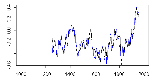
So MBH99$ignore2 relates to MBH98$sigma – what are the other columns? If you take the ratio of the MBH99$sigma to the MBH98$sigma, then there are only two “adjustments” – one for the period from 1400-1600 and one after 1600. The ratios are 1.187 and 1.643 respectively. Where do these come from? Who knows? I did this originally for the MBH98 comparison; Jean S responded that you could apply the above relationship between MBH98$sigma and the MBH99$ignore2 to extend this back to the first step. Using the constant, we get a ratio of 1.58 for the 1000-1399 step. These three values have something to do with the spectrum calculations of Mann and Less 1995, but what?

Figure 4. Top: black- MBH99 sigma; red – MBH98 sigma; bottom ratio of MBH99 sigma to MBH98 sigma (using the ignore2 to extend to 1000-1399).
A few comments from Jean S, as a statistics post-doc:
“these “climate scientists” seem to be a light year behind from my field in terms of understanding and using statistics, and their terminology is weird…
“what they are doing just does not make too much real sense (in the meaning of mathematics or statistics) … nor do I approve the thing.
“WTF!?!”
So I guess the “mask” is a complete ad-hoc, which is of course impossible to figure out. See what they say in MBH99, they don’t give any hint how they “take into account” different things (this usually means that procedure is completely ad-hoc). Also they say “to be conservative” which usually refers to some kind of ad-hoc number selection.
By the way, you should show all statisticians you happen to talk to Mann’s phrase “robustly estimated median” from caption~2 in MBH99. It must be one of the most unprecedentedly 😉 stupid phrases ever published in a scientific journal. Exactly this type of phrases I see from our under-grads with great ego but little understanding.
Update April 27, 2006: Jean S has emailed me to point out that the following holds exactly:
sum(MBH99$ignore1 ^2) + sum (MBH99$ignore2^2) = sum(MBH99$sigma^2)
So we have an orthogonal decomposition. Jean S proposes that this has something to do win the Mannian distinctive of “secular” frequencies. MBH99$ignore2^2 is almost exactly equal to (2/3)^2 * MBH98$sigma^2 in the overlap and is thus the standard error of the residuals weighted by 2/3 (or some high-frequency subset.) So it looks like some other series is weighted by 1/3 to get MBH99$ignore1. Ideas welcome. (End update).
May 6, 2006: Eduardo Zorita comments below re MBH99:
Well, the uncertainty limits in the paper (Fig 1) are 4 times smaller than in TAR, although they should be representing the same thing
Update: October 5, 2006
Jean S has observed that the MBH99 preprint (but not the final version) contained a graphic of the spectrum of residuals for the AD1820 and AD1000 networks (though as noted below, this may not be correct. Jean S’ digitization of the residuals is here AD1000 AD1820 . He used the Matlab routine for calculating MTM spectra script here , digital versions of spectra here AD1000 AD1820 . His emulation of MBH99 Figure 2 is here. Jean S’ emulation closely matches the corresponding figure from MBH99 preprint shown here.
Some new references:
- Allan Murphy: The Coefficients of Correlation and Determination as Measures of performance in Forecast Verification, Weather and Forecasting: Vol. 10, No. 4, pp. 681-688, December 1995.
- Michael Mann’s Lecture Notes for the course “Data Analysis in the Atmospheric Sciences”, available from here
Climategate postscript (Nov 3, 2023):
On July 31, 2003, (CG1 1059664704.txt) Tim Osborn wrote to Mann about the issue that Jean S addressed above:
I then looked at the file that I have been using for the uncertainties associated with MBH99 (see attachment), which I must have got from you some time ago. Column 1 is year, 2 is the “raw” standard error, 3 is 2*SE. But what are columns 4 and 5? I’ve been plotting column 4, labelled “1 sig (lowf)” when plotted your smoothed reconstruction, assuming that this is the error appropriate to low-pass filtered data. I’d also assumed that the last column “1 sig (highf)” was appropriate to high-pass filtered data. I also noticed that the sum of the squared high and low errors equalled the square of the raw error, which is nice.
One phrase from this email thread will be familiar to readers – this is the notorious “dirty laundry” email. It’s about confidence intervals.
p.s. I know I probably don’t need to mention this, but just to insure absolutely clarify on this, I’m providing these for your own personal use, since you’re a trusted colleague. So please don’t pass this along to others without checking w/ me first. This is the sort of “dirty laundry” one doesn’t want to fall into the hands of those who might potentially try to distort things…
Osborn observed:
From MBH99 it sounds like post-1600 you assume uncorrelated gaussian calibration residuals. In which case you would expect the errors for a 40-year mean to be reduced by sqrt(40). This doesn’t seem to match the values in the attached file. Pre-1600 you take into account that the residuals are autocorrelated (red noise rather than white), so presumably the reduction is less than sqrt(40), but some factor (how do you compute this?).
Osborn’s question here corresponds to the question in my post in which I had observed different adjustments from 1400-1600 and after 1600. (“If you take the ratio of the MBH99$sigma to the MBH98$sigma, then there are only two “adjustments” – one for the period from 1400-1600 and one after 1600. The ratios are 1.187 and 1.643 respectively.”) According to Osborn’s comment here, Mann assumed “uncorrelated gaussian calibration residuals” after 1600, but before 1600, Mann recognized that residuals were autocorrelated.
Mann then provided two possible “explanations” of the MBH sigmas: either as a combination “low f[requency]” and “high f[requency]” uncertainties, or as standard deviation of calibration residuals using “effective” degrees of freedom:
The one-sigma *total* uncertainty is determined from adding the low f and high f components of uncertainty in quadrature. The low f and high f uncertainties aren’t uncertainties for a particular (e.g. 30 year or 40-year) running mean, they are band integrated estimates of uncertainties (high-frequency band from f=0 to f=0.02, low-frequency band from f=0.02 to f=0.5 cycle/year) taking into account the spectrum of the residual variance (the broadband or “white noise” mean of which is the nominal variance of the calibration residuals) Alternatively, one could calculate uncertainties for a particular timescale average using the standard deviation of the calibration residuals, and applying a square-root-N’ argument (where N’ is the effective degrees of freedom in the calibration residuals). I believed I did this at one point, and got similar results.
Osborn then asked Mann how he computed the values:
I now understand how you compute them in theory. I have two further questions though (sorry):
(1) how do you compute them in practise? Do you actually integrate the spectrum of the residuals?
(2) how would I estimate an uncertainty for a particular band of time scales (e.g. decadal to secular, f=0.0 to 0.1)?If integrating the spectrum of the residuals, I wonder whether integrating from f=0 to f=0.02 and then f=0.02 to (e.g.) f=0.1 (note this last limit has changed) would give me the right error for time scales of 10 years and longer (i.e. for a 10-yr low pass filter)?
The way I had planned to do this was to assume the residuals could be modelled as a first order autoregressive process, with lag-1 autocorrelation r1=0.0 after 1600 (essentially white) and r1=??? before 1600. Do you know what the lag-1 autocorrelation of the residuals is for the network that goes back to 1000 AD?