PAGES2K Online “Journal Club”

I’m listening to a presentation by PAGES2K authors sponsored by Nature:

NPG journal club: How has Earth’s climate changed in the past 2,000 years? #NPGjclub

Started at 11 am Eastern.

11:30. Open for questions. I have submitted the following:

Can you explain the decision to label the article as only a “Progress Article”, rather than a Research Article?

Nature’s definition of Progress Articles http://www.nature.com/ngeo/authors/content_types.html says that such articles are “commissioned by the editors” and associates them with “fields that might not yet be mature enough for review”. It also states that such articles do not include received and accepted dates and places more restrictive word and display limits than full Research Articles:

“When the discussion is focused on a developing field that might not yet be mature enough for review, a Progress article is more appropriate. Progress articles are up to 2,000 words in length, with up to 4 display items (figures, tables or boxes). References are limited to 50. Reviews and Progress articles are commissioned by the editors, but proposals including a short synopsis are welcome. Reviews and Progress articles are always peer-reviewed to ensure factual accuracy, appropriate citations and scholarly balance. They do not include received/accepted dates.”

Thousand-year paleoclimate reconstructions clearly do not qualify as a “developing field… not mature enough for review”. So why was this article classified as only a Progress Article?

Did Nature editors either commission the PAGES2K article or receive a short synopsis from the authors?

Given the above policy against received and accepted dates, why did Nature you include received and accepted such dates for the PAGES article?

Here is my surmise on the matter. The PAGES2K article presents eight different reconstructions using a variety of methods. Each individual reconstruction warranted separate peer review in specialist literature and it was impossible within the required time frame for peer reviewers to provide the peer review expected of a Research Article. As a way out of the review dilemma, one or more reviewers suggested that PAGES2K be published as a Progress Article, a recommendation that you adopted, even though the article did not fit within the definition. Can you comment on this surmise?

Cook’s Survey

John Cook, whose crush on Lewandowsky continues unabated, asked various blogs, including Climat Audit, to direct readers to another online survey. Lucia has discussed the survey here.

The links to the survey from SKS here is http://survey.gci.uq.edu.au/survey.php?c=1R9YT8YMZTWF and from Rabett hereis http://survey.gci.uq.edu.au/survey.php?c=II7WP4R4VRU7. More IDs are available at Lucia’s.

It is easy enough to access both blogs using hidemyass.com and then click on their link to the survey. In the survey, readers are asked to rate various abstracts according to their support for AGW. I urge readers to take as much care with the survey as the respondents to Lewandowsky’s Hoax :), where Lewandowsky argued that fake responses should not be excluded.

More Kaufman Contamination

Kaufman and paleo peer reviewers ought to be aware that the recent portion of varve data can be contaminated by modern agriculture, as this was a contentious issue in relation to Mann et al 2008 (Upside Down Mann) and Kaufman et al 2009. Nonetheless, Kaufman et al 2013 (PAGES), despite dozens of coauthors and peer review at the two most prominent science journals, committed precisely the same mistake as his earlier article, though the location of the contaminated data is different.

The contaminated series is readily identified as an outlier through a simple inspection of the data. The evidence of contamination by recent agriculture in the specialist articles is completely unequivocal. This sort of mistake shouldn’t be that hard to spot even for real climate scientists.

. Continue reading

PAGES2K: Gifford Miller vs Upside-Down Kaufman

The PAGES2K Arctic reconstruction uses Gifford Miller’s Hvitavatn (Iceland) data upside down. The error “matters” because this series is one of rather few PAGES2K series that show a Hockey Stick. Such gross errors ought to be corrected before the data is cited for policy purposes or said to confirm previous studies.

Continue reading

Steig’s Bladeless “Hockey” Stick

In a recent RC post entitled “Ice Hockey” and a recent Nature article, Steig and coauthors have introduced a novel and very baroque “hockey stick”, one without a blade. A true Halloween of horrors: in addition to Gergis’ zombie hockey stick, the bladeless Hockey Stick of Sleepy Hollow is now at large.

The appearance of Steig’s bladeless hockey stick was apparently so horrifying that he dared not show it in the RC post. However, I believe that CA readers are made of sterner stuff and will be able to withstand the sight of even a bladeless hockey stick, which is shown below. Continue reading

Non-centring in the Forest 2006 study

This is a cautionary tale, about a mystery that had an unexpected explanation. It’s not intended as a criticism of the scientists involved, and the problem involved, although potentially serious, actually had little impact on the results of the study concerned. However, I am hopeful that mathematically and computing orientated readers will find it of interest. But first I need to give some background information.

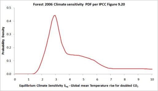
Forest et al. 2006 (F06), here, was a high profile observationally-constrained Bayesian study that estimated equilibrium climate sensitivity (Seq) simultaneously with two other key climate system parameters / properties, ocean effective vertical diffusivity (Kv) and aerosol forcing (Faer). Both F06 and its predecessor Forest 2002 had their climate sensitivity PDFs featured in Figure 9.20 of the AR4 WG1 report. I started investigating F06 in 2011, with a view to using its data to derive estimated climate system parameter PDFs using an objective Bayesian method.  That work eventually led to my paper ‘An objective Bayesian, improved approach for applying optimal fingerprint techniques to estimate climate sensitivity’, recently published in Early online release form by Journal of Climate, here.

Readers may recall that I found some basic statistical errors in the F06 code, about which I wrote a detailed article at Climate Audit, here. But those errors could not have affected any unrelated studies.  In this post, I want to focus on an error I have discovered in F06 that is perhaps of wider interest. The error has a source that will probably be familiar to CA readers – failure to check that data is zero mean before undertaking principal components analysis (PCA) / singular value decomposition (SVD).

The Forest 2006 method
First, a recap of how F06 works. It uses three ‘diagnostics’  (groups of variables whose observed values are compared to model-simulations): surface temperature averages from four latitude zones for each of the five decades comprised in 1946–1995; deep ocean 0–3000 m global temperature trend over 1957–1993; and upper air temperature changes from 1961–80 to 1986–95 at eight pressure levels for each 5-degree latitude band (8 bands being without data). AOGCM unforced long control run data is used to estimate natural, internal variability in the diagnostic variables. The MIT 2D climate model, which has adjustable parameters calibrated in terms of  Seq , Kv and Faer, was run several hundred times at different settings of those parameters, producing sets of model-simulated temperature changes on a coarse, incomplete, grid of the three climate system parameters.

A standard optimal fingerprint method, as used in most detection and attribution (D&A) studies to deduce anthropogenic influence on the climate, is employed in F06. The differences between changes in model-simulated and observed temperatures are ‘whitened’, with the intention of making them independent and all of unit variance. Then an error sum-of-squares, r2, is calculated from the whitened diagnostic variable differences and a likelihood function is computed from r2, on the basis of an appropriate F-distribution. The idea is that, the lower r2 is, the higher the likelihood that the model settings of Seq, Kv and Faer correspond to their true values. Either the values of the model-simulated diagnostic variables are first interpolated to a fine regular 3D grid (my approach) or the r2 values are so interpolated (the F06 approach). A joint posterior PDF for Seq, Kv and Faer is then computed, using Bayes’ rule, from the multiplicatively-combined values of the likelihoods from all three diagnostics and a prior distribution for the parameters. Finally, a marginal posterior PDF is computed for each parameter by integrating out (averaging over) the other two parameters.

The whitening process involves a truncated inversion of the estimated (sample) control-run data covariance matrix. First an eigendecomposition of that covariance matrix is performed. A regularized inverse transpose square root of that matrix is obtained as the product of the eigenvectors and the reciprocal square roots of the corresponding eigenvalues, only the first k eigenvector–eigenvalue pairs being used. The raw model-simulation – observation differences are then multiplied by that covariance matrix inverse square root to give the whitened differences. As many readers will know, by setting the number of retained eigenfunctions or EOFs (eigenvector-patterns), k affects how much detail is retained upon the inversion of the covariance matrix. The higher the truncation parameter k, the more detail is retained and the better is discrimination between differing values of Seq, Kv and Faer. However, if k is too high then the likelihood values will be heavily affected by noise and potentially very unrealistic. There is a standard test, detailed in Allen and Tett 1999 (AT99), here, that can be used to guard against k being too high.

The Forest 2006 upper air diagnostic: effect of EOF truncation and mass weighting choices
My concern in this article is with the F06 upper air (ua) diagnostic. F06 weighted the upper air diagnostic variables by the mass of air attributable to each, which is proportional to the cosine of its mean latitude multiplied by the pressure band allocated to the relevant pressure level. The weighting used only affects the EOF patterns; without EOF truncation it would have no effect. It seems reasonable that each pressure level’s pressure band should be treated as extending halfway towards the adjacent pressure levels, and to surface pressure (~1000 hPa) at the bottom. But where to treat the top end of the pressure band attributable to the highest, 50 hPa pressure level, as being is less clear. One choice is halfway towards the top of the atmosphere (0 hPa). Another is halfway towards 30 hPa, on the grounds that data for the 30 hPa level exists – although it was excluded from the main observational dataset due to excessive missing data. The F06 weighting was halfway towards 30 hPa. The weighting difference is minor: 4.0% for the 50 hPa layer on the F06 weighting, 5.6% on the alternative weighting.

However, it turns out that the fourteenth eigenvector – and hence the shape of the likelihood surface, given the F06 choice of kua = 14 –  is highly sensitive to which of these two mass-weighting schemes is applied to the diagnostic variables, as is the result from the AT99 test.  Whatever the physical merits of the two 50 hPa weighting bases, the F06 choice appears to be an inferior one from the point of view of stability of inference. It results, at kua = 14, in failure of  the recommended, stricter, version of the AT99 test, and a likelihood surface that is completely different from that when kua = 14 and the alternative weighting choice is made (which well satisfies the AT99 test). Moreover, if  kua is reduced to 12 then whichever weighting choice is made the AT99 test is satisfied and the likelihood surface is similar to that at kua = 14 when using the higher alternative, non-F06, 50 hPa level weighting.

AT99 test results
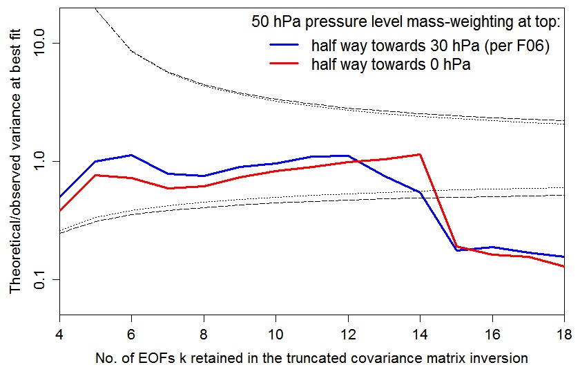
The below graph plots the AT99 test values – the ratio of the number of degrees of freedom in the fit to the r2 value at the best fit point, r2min, for the two 50 hPa weightings. To be cautious, the value should lie within the area bounded by the inner, dotted black lines (which are the 5% and 95% points of the relevant chi-squared distribution). The nearer it is to the unity, the better the statistical model is satisfied.

best-fit-consistency.ua

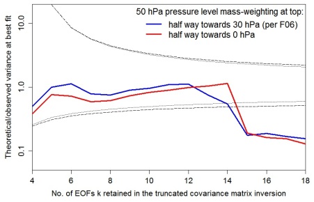
Using the F06 50 hPa level weighting, at kua = 13 the AT99 test is satisfied (although less well than at kua = 12), and the likelihood surface is more similar to that – using the same weighting – at kua = 12 than to that at kua = 14.

Upper air diagnostic likelihood surfaces
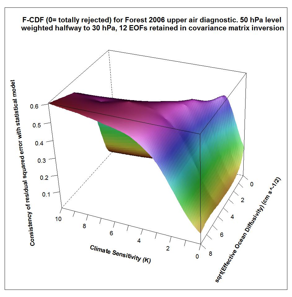
The following plots show what the upper air diagnostic likelihood consistency surface looks like in {Seq, Kv} space using the F06 50 hPa level weighting, at successively kua = 12, kua = 13 and kua = 14. Faer  has been integrated out, weighted by its marginal PDF as inferred from all diagnostics. The surface is for the CDF, not the PDF. It shows how probable it is that the upper air diagnostic r2 value at each {Seq, Kv} point could have arisen by chance, given the estimated noise covariance matrix. Note that the orientation of the axes is non-standard.

like.ua.s2.64k12.39.FnaNew

like.ua.s2.64k13.39.FnaNew

like.ua.s2.64k14.39.FnaNew

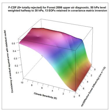
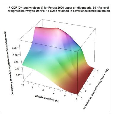
Notice that the combination of high climate sensitivity but fairly low ocean diffusivity is effectively ruled out by the kua = 12 likelihood surface, but not by the kua = 14 surface nor (except somewhere below sqrt(Kv) = 2) by the kua = 13 surface. It is the combination of high climate sensitivity but moderately low ocean diffusivity that the F06 surface and deep ocean diagnostics, acting together, have difficulty well-constraining. So the failure of the upper air diagnostic to do so either fattens the upper tail of the climate sensitivity PDF.

Why didn’t the Forest 2006 upper air r2 values reflect kua = 14, as used?
I couldn’t understand why, although F06 used kua = 14, the pattern of its computed r2 values, and hence the likelihood surface, were quite different from those that I computed in R from the same data. Why should the F06 combination of kua = 14 and 50 hPa level weighting produce one answer when I computed the r2 values in R, and a completely different one when computed by F06’s code? Compounding the mystery, the values produced by the F06 code seemed closely related to the kua = 13 case.

I could explain why each F06 r2 would only be only 80% of its expected value, because the code F06 used was designed for a different situation and it divides all the r2 values by 1.25. The same unhelpful division by 1.25 arises in F06’s computation of the r2 values for its surface diagnostic.  But even after adjusting for that, there were large discrepancies in the upper air r2 values. I thought at first that it might be something to do with IDL, the rather impenetrable language in which all the F06 code is written, having vector and array indexing subscripts that start at 0 rather than, as in R, at 1. But the correct explanation was much more interesting.

A missing data mask is generated as part of the processing of the observational data, based on a required minimum proportion of data being extant. That mask may have been used to mark what points should be treated as missing in the (initially complete) control data, when processing it to give changes from the mean of each twenty year period to the mean of a ten year period starting 25 years later. In any event, the values of the 80–85°N latitude band, 150 and 200 hPa level diagnostic variables, along with the variables for a lot of other locations, are marked as missing in the processed control data temperature changes matrix, by being given an undefined data marker value of ‑32,768°C. Such use of an undefined data marker value is common practice for external data, although not being an IDL acolyte I was initially uncertain why it was employed within IDL. It turns out that, when the code was written, IDL did not have a NaN value available.

Rogue undefined data maker values
Variables in the processed control data are then selected using a missing values mask derived from the actual processed observational data, which should eliminate all the control data variables with ‘undefined data’ marker values . Unfortunately, it turns out that the two 80–85°N latitude band control data variables mentioned, unlike all the other control data variables marked as missing by having ‑32,768°C values, aren’t in fact marked as missing in the processed observational data. So they get selected from the control data along with the valid data. I think that the reason why those points aren’t marked as missing in the observational data could possibly be linked to what looks to me like a simple coding error in a function called ‘vltmean’, but I’m not sure.  (All the relevant data and IDL code can be downloaded as large (2 GB) file archive GRL06_reproduce.tgz here.)

So, the result is that the ‑32,768°C control data marker values for the 80–85°N latitude band, 150 and 200 hPa pressure levels get multiplied by the cosine of 82.5° (the mid-point of the latitude band) and then by pressure-level weighting factors of respectively 0.05 and 0.075, to give those variables weighted values of ‑213.854°C and ‑320.781°C for all rows of the final, weighted, control data matrix.  Here’s an extract, at the point it is used to compute the whitening transformation, from the first row of the weighted control data matrix, CT1WGT, resulting from running the F06 IDL code, with the rogue data highlighted:

-0.0013 -213.8540   0.0127    0.0094     0.0051     0.0047     0.0056     0.0024     0.0005          0.0011
0.0038       0.0115     0.0125     0.0058     0.0060    0.0046      0.0030    0.0016     0.0000        -0.0002
0.0036       0.0077    0.0069     0.0001   -0.0047    -0.0060    -0.0067    -0.0050    -0.0030    -320.7810

I should say that I have been able to find this out thanks to considerable help from Jonathan Jones, who has run various modified versions of the F06 IDL code for me. These output relevant intermediate data vectors and matrices as text files that I can read into R and then manipulate.

Why does the rogue data have any effect?
Now, the control data contamination with missing data marker values doesn’t look good, but why should it have any effect? A constant value in all rows of a column of a matrix gives rise to zero entries in its covariance matrix, and a corresponding eigenvalue of zero, which – since the eigenvalues are ordered from largest to smallest – will result in that eigenfunction being excluded upon truncation.

But that didn’t happen. The reason is as follows. F06 used existing Detection and Attribution (D&A) code in order to carry out the whitening transformation – an IDL program module called ‘detect’.  That appears to be a predecessor of the standard module ‘gendetect’, Version 2.1, available at The Optimal Detection Package Webpage, which I think will have been used for a good number of published Detection and Attribution studies. Now, neither detect nor gendetect v2.1 actually carries out an eigendecomposition of the weighted control data covariance matrix.  Instead, they both compute the SVD of the weighted control data matrix itself. If all the columns of that matrix had been centred, then the SVD eigenvalues would be the square roots of the weighted control data sample covariance matrix eigenvalues, and the right singular vectors of the SVD decomposition would match that covariance matrix’s eigenvectors.

However, although all the other control data columns are pretty well centred (their means are within ± 10% or so of their – small – standard deviations), the two columns corresponding to the constant rogue data values are nothing like zero-mean. Therefore, the first eigenfunction  almost entirely represents a huge constant value for those two variables, and has an enormous eigenvalue. The various mean values of other variables, tiny by comparison, will also be represented in the first eigenfunction. The reciprocal of the first eigenvalue is virtually zero, so that eigenfunction contributes nothing to the r2 values. The most important non-constant pattern, which would have been the first eigenfunction of the covariance matrix decomposition, thus becomes the second SVD eigenfunction. There is virtually perfect equivalence between the eigenvalues and eigenvectors, and thus the whitening factors derived from them, of the SVD EOFs 2–14 and (after taking the square root of the eigenvalues) those of the covariance matrix eigendecomposition EOFs 1–13. So, although F06 ostensibly uses kua=14, it effectively uses kua =13. Mystery solved!

Concluding thoughts
It’s not clear to me whether, in F06’s case, the combination of arbitrary marker values incorrectly getting through the mask and then dominating the SVD had any further effects. But it is certainly rather worrying that this could happen. Is it possible that, without centring, the means of a control data matrix could give rise to a rogue EOF that did affect the r2 values, or otherwise materially distort the EOFs, in the absence of any masking error? If that did occur, might the results of some D&A studies be unreliable? Very probably not in either case. However, it does show how careful one needs to be with coding, and importance of making code as well as data available for investigation.

There was actually a good reason for use of the SVD function (from the related PV-wave language, not from IDL itself) rather than the IDL PCA function, which despite its name does actually compute the covariance matrix. Temperature changes in an unforced control run have a zero mean expectation, provided drifting runs are excluded. Therefore, deducting the sample mean is likely to result in a less accurate estimate of the control data covariance matrix than not doing so (by using the SVD eigendecomposition, or otherwise). However, the downside is that if undefined data marker values are used, and something goes wrong with the masking, the eigendecomposition will be heavily impacted. Version 3.1 of gendetect v3.1 does use the PCA function, so the comments in this post are not of any possible relevance to recent studies that use the v3.1 Optimal Detection Package code. However, I suspect that Version 2.1 is still in use by some researchers.

So, the lesson I draw is that use within computer code of large numbers as marker values for undefined data is risky, and that an SVD, rather than a eigendecomposition of the covariance matrix, should only be used to obtain eigenvectors and eigenvalues if great care is taken to ensure that all variables are in fact zero mean (in population, expectation terms).

Finally, readers may like to note that I had a recent post at Climate Etc, here, about another data misprocessing issue concerning the F06 upper air data. That misprocessing appears to account for the strange extended shoulder between 4°C and 6°C  in F06’s climate sensitivity PDF, shown below.

Nic Lewis

F06 Fig9.20


PAGES2K Reconstructions

The PAGES2K article to be published tomorrow will show eight regional reconstructions, which are plotted below. In today’s post, I’ll try to briefly summarize what, if anything, is new about them.

pages reconstructions

Antarctica: This is a composite of 11 isotope series (mostly d18O). It includes some new data (e.g. Steig’s new WAIS series) and some long unavailable data (Ellen Mosley-Thompson’s Plateau Remote). It shows a long-term decline with nothing exceptional in the 20th century. Steig has recently characterized the recent portion of Antarctic isotope as “unusual”, but this is really stretching the facts to the point of disinformation. I’ll post separately on this.

Arctic: This is a somewhat expanded version of the Kaufman data, unsurprising since Kaufman seems to have been the leader of the program. It shows an increase from 1800 to 1950, with leveling off since 1950. Its modern values are higher than medieval values. It is heavy on varvology (22 varve series), but, like Kaufman et al, also has ice cores (16) and tree rings (13, including Briffa’s Yamal) plus a few others. They use Korttajarvi, but Kaufman has issued one correction on this already in 2009 and avoided use of the contaminated portion. We’ve discussed Arctic d18O values from time to time, observing that their 20th century values are rather unexceptional. My surmise is that the varve data, which, as discussed in other CA threads, is highly problematic, is the main contributor to the modern-medieval differential in the PAGES reconstruction.

Asia: This reconstruction is based entirely on tree rings (229 series), all, interestingly, used in a positive orientation. 20th century values are elevated but the reconstruction lacks the distinctive blade of, for example, the Gergis stick. The majority of the tree ring data is unarchived: chronologies have been included in the PAGES2K data, but the underlying measurement remains unarchived.

Australia: this is the Gergis reconstruction. There are only two long series (both tree ring). As is well known, Gergis picked data according to ex post correlation to temperature (contrary to the representation in the disappeared article). The present network is little changed from the network in the disappeared article, with the precise differences remaining to be explained. The network is about half tree ring data and about half is short coral (nearly all O18) data. The blade in the Gergis stick comes almost entirely from coral O18 data – for which corresponding medieval information is lacking. The reconstruction is thus a sort-of splice of low-amplitude tree ring data with high amplitude coral O18. Coral specialist literature nearly always uses Sr data as a measure of temperature. The 20th century increase in coral Sr data is much less than O18 data: however, Gergis screened out the Sr data and almost exclusively used coral O18 data.

Europe: The network is 10 tree ring series and one documentary. I don’t know at present how the series were chosen. Most of the increase in the reconstruction took place prior to 1950. Late 20th century values equal and then exceed mid-century values. It will be interesting to see whether sustained ring widths will be maintained with these particular chronologies during warmer temperatures.

North America.
There are two North American reconstructions. A reconstruction using pollen is at 30 year intervals and ends in 1950. It shows elevated temperatures in the late first millennium that exceed the most recent values in the series. The other reconstruction uses tree rings. It includes many series from the MBH98 dataset, including the Graybill bristlecone chronologies. Although the tree ring data is accurately dated, the reconstruction is only reported at 10-year intervals. Although the data set includes new data reaching into the present century, the reconstruction is shown only to 1974.

South America: This network is particularly hard to understand. It shows particularly low medieval values relative to the modern period – a point that is relevant to assertions on medieval-modern differential. The network also uses intrumental data. It has two long ice core series from Quelccaya, which, as previously noted, appear (according to the SI) to have been inverted, a decision which, if correct, would rather detract from conclusions about modern-medieval differential drawn from this reconstruction, given that the medieval portion of the reconstruction only has a few contributors, of which Quelccaya is prominent.

PAGES2K South America

A commenter observed that the forthcoming PAGES2K received over 50 pages of review comments from one reviewer. One wonders what he had to say about the PAGES2K South American network which has some very odd characteristics.

Here is a list of proxies with a couple of interesting features highlighted.

soamer network

First, note that the “proxy” network includes four instrumental records, which seems to be peeking at the answer if the “skill” of the early portion of the reconstruction is in any way assessed on the ability of the network (including instrumental) to estimate instrumental temperature.

Second, one-third of the tree ring series are inverted. Is this an ex ante relationship or mere ex post correlation? We’ll find out eventually, I guess.

Finally, the two longest series are from Quelccaya, a site that we’ve regularly discussed. In the PAGES reconstruction, the d18O values are said to have been inverted. If this is how they actually used the data, as opposed to an error in the SI, it will be a surprise. A quick reverse engineering check indicates that the d18O orientation is inverted (A multiple correlation of recon against proxies in the 857-963 period.)

The PAGES2K Quelccaya version is different from any other Thompson version (as usual.) The graphic below compares the PAGES version (ending in 1995) with the PNAS version (archived in 2006) and the most recent (2013) version. The PAGES version has a sharp downtick in the late 1980s that was not reported in the PNAS version (ending in 1997) or in the 2013 version, though earlier aspects of the graphic cohere. Where did the new version come from? With Thompson, these inconsistencies are the rule, rather than the exception. If Thompson’s data is to be used by IPCC, every damn sample and measurement should be archived so that there is an audit trail.

quelccaya versions

PAGES2K, Gergis and Made-for-IPCC Journal Articles

March 15, 2013 was the IPCC deadline for use in AR5 and predictably a wave of articles have been accepted. The IPCC Paleo chapter wanted a graphic on regional reconstructions and the PAGES2K group has obligingly provided the raw materials for this graphic, which will be published by Nature on April 21. Thanks to an obliging mole, I have information on the proxies used in the PAGES2K reconstructions and will report today on the Gergis reconstruction, of interest to CA readers, which lives on a zombie, walking among us as the living dead.

The PAGES2K article has its own interesting backstory. The made-for-IPCC article was submitted to Science last July on deadline eve, thereby permitting its use in the Second Draft, where it sourced a major regional paleo reconstruction graphic. The PAGES2K submission used (in a check-kited version) the Gergis reconstruction, which it cited as being “under revision” though, at the time, it had been disappeared.

The PAGES2K submission to Science appears to have been rejected as it has never appeared in Science and a corresponding article is scheduled for publication by Nature. It sounds like there is an interesting backstory here: one presumes that IPCC would have been annoyed by Science’s failure to publish the article and that there must have been considerable pressure on Nature to accept the article. Nature appears to have accepted the PAGES2K article only on IPCC deadline eve.

The new PAGES2K article contains reconstructions for all continents and has an extremely long list of proxies, some of which have been discussed before, but some only now making their first digital appearance. Each regional reconstruction is a major undertaking and deserving of separate peer review. It seems impossible that these various regional reconstructions could themselves have been thoroughly reviewed as re-submitted to Nature. Indeed, given that the PAGES2K coauthor list was very large, one also wonders where they located reviewers that were unconflicted with any of the authors.

Of particular interest to CA readers is the zombie version of the Gergis reconstruction. Previous CA articles are tagged gergis.

CA readers will recall that Gergis et al 2012 had stated that they had used detrended correlations to screen proxies – a technique that seemingly avoided the pitfalls of correlation screening. Jean S pointed out that Gergis et al had not used the stated technique and that the majority of their proxies did not pass a detrended correlation test – see CA discussion here (building on an earlier thread) reporting that only 6 of 27 proxies passed the stated significance test.

Senior author David Karoly asked coauthor Neukom to report on correlations and, after receiving Neukom’s report, wrote his coauthors conceding the validity of the criticism:

Thanks for the info on the correlations for the SR reconstructions during the 1911-90 period for detrended and full data. I think that it is much better to use the detrended data for the selection of proxies, as you can then say that you have identified the proxies that are responding to the temperature variations on interannual time scales, ie temp-sensitive proxies, without any influence from the trend over the 20th century. This is very important to be able to rebut the criticism is that you only selected proxies that show a large increase over the 20th century ie a hockey stick .

The same argument applies for the Australasian proxy selection. If the selection is done on the proxies without detrending ie the full proxy records over the 20th century, then records with strong trends will be selected and that will effectively force a hockey stick result. Then Stephen Mcintyre criticism is valid. I think that it is really important to use detrended proxy data for the selection, and then choose proxies that exceed a threshold for correlations over the calibration period for either interannual variability or decadal variability for detrended data. I would be happy for the proxy selection to be based on decadal correlations, rather than interannual correlations, but it needs to be with detrended data, in my opinion. The criticism that the selection process forces a hockey stick result will be valid if the trend is not excluded in the proxy selection step.

Unfortunately, as coauthor Neukom immediately recognized a big probleM:

we don’t have enough strong proxy data with significant correlations after detrending to get a reasonable reconstruction.

Mann and Schmidt immediately contacted Gergis and Karoly advising them to tough it out as Mann had done with his incorrect use of the contaminated portion of the Tiljander data, where Mann’s refusal to concede the error had actually increased his esteem within the climate community. Nonetheless, Gergis and Karoly notified Journal of Climate of the problem. Despite Karoly’s concerns about substantive problems, Gergis hoped to persuade Journal of Climate that the error was only in their description of methodology and to paper over the mistake. However editor Chiang’s immediate reaction was otherwise, advising Gergis:

it appears that you will have to redo the entire analysis (and which may result in different conclusions), I will also be requesting that you withdraw the paper from consideration.

Upon receiving advice from Mann, Gergis tried to persuade Journal of Climate that the error was not one of methodology, but one of language only. Bur Chief Editor Broccoli was not persuaded, responding:

In that email (dated June 7) you described it as “an unfortunate data processing error,” suggesting that you had intended to detrend the data. That would mean that the issue was not with the wording but rather with the execution of the intended methodology.

Editor Chiang added:

Given that you had further stated that “Although it was an unfortunate data processing error, it does have implications for the results of the paper,” we had further took this to mean that you were going to redo the analysis to conform to the description of the proxy selection in the paper.

After further lobbying form Gergis, Chiang reluctantly permitted Gergis to re-submit as a “revision” by the end of July, but insisted that they show the results of both methods, describing this as an “opportunity” to show the robustness of their work:

In the revision, I strongly recommend that the issue regarding the sensitivity of the climate reconstruction to the choice of proxy selection method (detrend or no detrend) be addressed. My understanding that this is what you plan to do, and this is a good opportunity to demonstrate the robustness of your conclusions.

Gergis didn’t meet the July 31 deadline and Journal of Climate reported that the paper had been “withdrawn” by the authors.

The article was apparently resubmitted to Journal of Climate by the end of September, where, according to Gergis’ current webpage, it remains “under review”.

Nonetheless, the Gergis reconstruction has already been incorporated into the PAGES2K made-for-IPCC composite. CA readers will recall the Mole Incident in 2009. Once again, I am in possession of the proxy list used in the zombie reconstruction and can report that it has had only negligible changes.

On the left is a list of the 28 proxies used in the disappeared Gergis version, highlighting the proxies re-used in the zombie version. On the right is the list of proxies in the new version, highlighting the additions. 21 of 27 proxies are re-used. Six proxies have been excluded, while seven have been added. Remarkably, Gergis has kept the numbering as close as possible to the original list, so that the first 20 re-used proxies appear in the same order as in the original table.

gergis2012-table1 cropped

gergis2013- cropped

The medieval portion of their reconstruction only has two proxies – as observed at CA very early here, where it was also pointed out that these two proxies did not constitute “new” information, as claimed in an IPCC draft, since they had not only been available for AR4 but illustrated in it.

Excluded from the original list are a tree ring series(Takapari), two ice core series (both from Vostok) and three coral series (Bali, Maiana and Fiji 1F O18), replaced by a speleothem (Avaiki), three tree ring series (Baw Baw, Celery Top West, Moa Park), two coral luminescence series (Great Barrier Reef, Havannah) and a coral O18 series (Savusavu). None of the excluded or included series is particularly long.

Obviously Gergis et al have not “redone the analysis to conform to the description of the proxy selection in the paper” as they continue to use many of the proxies that failed the original significance test – see the graphic below from last June.

Nature reviewers obviously didn’t have the concerns about robustness that were expressed by Journal of Climate editors last summer, as the new article doesn’t demonstrate any such “robustness”. It will be interesting to see whether Journal of Climate editors will themselves adhere to the scruples that they showed last summer and require Gergis et al to demonstrate the robustness of their reconstruction.

The Hockey Team and Reinhart-Rogoff

As some readers have observed, there is a lively controversy regarding an influential recent paper by Reinhart and Rogoff. Herndon et al (of Raymond Bradley’s UMass-Amhertst) concluded that RR’s conclusions depended on a bad weighting method, inexplicable exclusion of data from certain countries and years and even an Excel coding error. All the sorts of issues that are familiar with Mann and the Hockey Team. Even the defences from Reinhart and Rogoff are eerily similar: no errors ever seem to “matter” because of some new and unfisked study. One big difference: Reinhart and Rogoff at least conceded things that were unarguable, whereas Mann and the Hockey Team concede nothing, not even things as incontrovertible as upside down use of contaminated data.

See here here here here here

. Continue reading